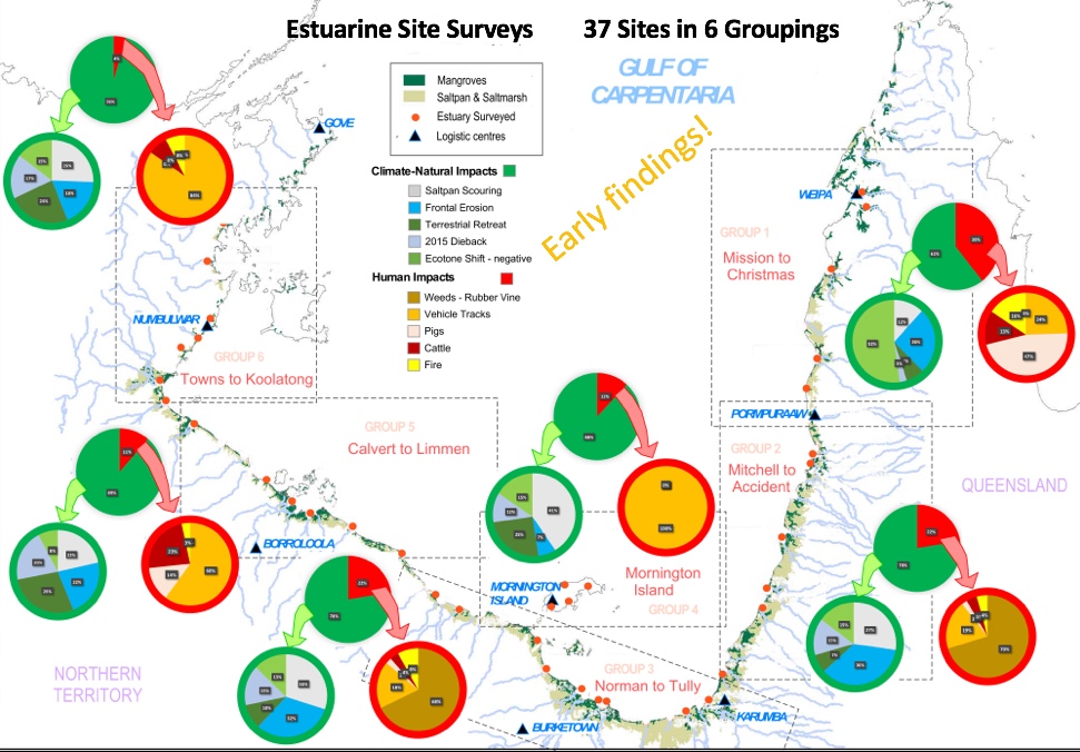
The major estuaries and their tidal wetlands of the Gulf of Carpentaria were impacted by mass dieback of mangroves in 2015-2016. To assess the full extent of the dieback and the major changes in the wetland areas, surveys in 2017 and 2019 were conducted along 31–37 major estuary mouths. Methods: The estuary surveys were conducted during aerial surveys using the same methods generally (see associated metadata record for more details: Gulf of Carpentaria Mangrove Aerial Shoreline Surveys 2017 & 2019 (NESP TWQ 4.13, JCU)). Shoreline edges were filmed and observations scored within a few kilometres of each estuary mouth. The observations recorded included a standard set of 10-20 features related to natural and human associated pressures like storm impacts, shoreline erosion, 2015 dieback of mangroves, fire damage, feral pig damage plus roads and buildings. Observations were summarised for each factor based on extent and severity scores to provide respective rankings of influence. These observations were further linked to respective likely drivers like sea level rise, storm winds, rough seas, plus the human associated ones of fire, pigs and weeds. The surveys collected observational data to classify the state, condition and health of the shoreline using criteria: 1. Driver type: list the drivers of change observed 2. Indicator: the indicator observed 3. Habitat: listing of the tidal wetland habitats affected 4. Extent: estimate the proportion of the tidal wetland affected 5. Severity: estimate severity of impact – time to natural recovery and effect on ecosystem function/structure 6. Time frame: when did the impact occur 7. Observations: notes and other comments These strategies were used to evaluate habitat condition associated with particular drivers, as well as providing an evaluation of local and national management priorities. The follow criteria were used to score the extent, severity and time frame (where applicable) for the criteria: Variable: Extent of impact on the tidal wetlands – The extent of tidal wetlands impacted determined by the proportional area showing impact. Impact extent assessment scoring criteria: 1. 1 – 10% 2. 10 – 30% - around 25% 3. 30 – 60% - around 50% 4. 60 – 90 % - around 75% 5. >90% Assessment metric: Extent score – extent of impact in the tidal wetlands Variable: Severity of impact on tidal wetland area – the severity of tidal wetlands impacted as determined by the degradation state observed. Impact severity assessment scoring criteria: 1. None – present but no observable effect 2. Minor – recovery within less than one year 3. Moderate – recovery over 1 – 2 years 4. Major – recovery over 2 – 10 years 5. Severe – recovery unlikely – collapse/replace Assessment metric: Severity score – severity of impact in the tidal wetlands Variable: Time frame of the impact on tidal wetland area – The timing of the impact on tidal wetlands as determined by the recovery potential observed. Impact time frame Assessment scoring criteria: 1. No observable effect, but potentially so 2. Current – now 3. Recent – less than 2 years ago 4. 4. Old – 2- 10 years ago 5. Very old - >10 years Assessment metric: Time frame score – time of occurrence of impact affecting tidal wetland area. Limitations of the data: Format of the data: This data consists of the survey assessment sheets from each estuary (xlsx) plus summary spreadsheets for each survey year. Each survey assessment sheet presents the original scores for Extent and Severity for each of the variables, as well as the calculations for respective rankings of influence. Note - The rankings of influence was used for the basis of the map visualisation by eAtlas, presenting the combined summary for each survey year as a shapefile. Data dictionary: 2019 Gulf of Carpentaria Tidal Wetland Threat Assessment Sheets: The extent, severity, time frame, restoration potential and other observations were collected for each of the following variables: Human Related Variable Driver Type: Indicator / Habitat Structure Loss: rock walls, wharf, ramps, roads / any zone Direct Loss: clearing, dead trees, landfill / any zone Altered Hydrology: bunds, drains, impoundments / higher zones mostly Encroachment: no buffer, cut-off flows / upper edge zone Access Tracks: wheel tracks, foot paths / Salt pans + high tide margin Stock Impacts: cattle, horses, goats – tracks / Salt pans + high tide margin Feral Damage: pigs, wallows, digging and tracks / Salt pan mangrove + freshwater wetlands Pollutant impact: oil spill, scum, dump, dieback / any zone Nutrient Excess: enhanced growth, expansion / any zone Fire Scorch: burnt vegetation - grass, dieback, blackened / upper margin - fringing zone Weed Smother: smothering weeds present / Beach ridge veg - mangrove upper edges Climate-natural Variable Driver Type: Indicator / Habitat Storm Damage: broken stems, damaged canopies, dead trees / mangrove closed canopies Shoreline erosion: fallen trees, steep bank, dieback / seaward + main channel edge stands of mangroves Root Burial: dead trees, burying sediments /shoreline and sea edge mangroves Inner Fringe Collapse: patchy dieback, canopy gaps / waters edge canopies Bank Erosion: channel edges eroded, fallen trees, steep / lower estuary banks Pan Scouring: upper pan, eroded edges, sheet erosion / upper salt pans Ecotone Shift -ve: dead trees pan edges / saltpan – mangrove Ecotone Shift +ve: new growth – seedlings, saplings / saltpan – mangrove Depositional gain: new growth – seedlings, saplings / waters edge margins Terretrial Retreat: dead terrestrial edge trees, eroded edge /terrestrial fringe Light gaps: dead trees, circular patch / mangrove closed canopies Altered hydrology: impounded, ponded water, dead trees /shoreline and sea edge mangroves 2015 Dieback: dead trees on back front edge / rear of mangrove front 2017 Gulf of Carpentaria Tidal Wetland Threat Assessment Sheets: Driver Type: Indicator / Habitat Pigs: wallows, pigs and tracks / inner mangrove + freshwater wetlands Fire: burnt vegetation – grass / Terrestrial margin - fringing mangroves Vehicle tracks: wheel tracks / Salt pans + high tide edge Cattle: cattle and tracks / Salt pans + high tide edge Weeds: weed species present / Beach ridge veg. / to mangrove upper edges 2015 Dieback: dead trees on pan edges / mangrove closed canopies Ecotone Shift: dead trees on pan edges / AM + Ceriops closed canopies Terretrial Retreat: dead terrestrial edge trees / Terrestrial fringe Saltpan scouring: eroded edges – escarpments / upper saltpans Light gaps: dead trees in a small circular patch / mangrove closed canopies Storm Damage: damaged canopies, dead trees / Mangrove closed canopies Depositional gain: new growth - seedlings. Saplings / waters edge margins Shoreline erosion: inner fringe collapse / seaward + main channel edge stands of mangroves Bank Erosion: channel edges eroded / lower estuary banks Altered hydrology: impounded, ponded water, dead trees / shoreline and sea edge mangroves Root Burial: dead trees and mobile sediments / shoreline and sea edge mangroves Note in some cases similar terminology was used for the same attribute for the different survey years, i.e. Access Tracks = Vehicle tracks, Stock impacts = cattle, Feral Damage = pigs. Data Dictionary - Shapefile Attributes Shapefile Attributes / Data Attribute: Description CATCHMENT/CATCHMENT: Catchment name. Estuaries are grouped in catchment areas described in the CSIRO Northern Australia Sustainable Project [CSIRO (2009) Water in the Gulf of Carpentaria Drainage Division. A report to the Australian Government from the CSIRO Northern Australia Sustainable Yields Project. CSIRO Water for a Healthy Country Flagship, Australia. xl + 479pp] SITE_NO/SITE_NO Number allocated to the site NAME/LOCATION_NAME: Location name REPEAT SURVEY/REPEAT SURVEY: whether the survey was repeated in 2019 (Y) or not (N) LATITUDE/LATITUDE: Latitude of the survey location. Coordinates mark the location of each estuary mouth. LONGITUDE/LONGITUDE: Longitude of the survey location. Coordinates mark the location of each estuary mouth. MANGROVE_S/MANGROVE_SPP_NO: Number of observed mangrove species for the location. S19-HUMAN/HUMAN_ISSUES: Total score of all Human threat issues for the 2019 survey assessment. Indicates the combined entent and severity scores across all the human issues and gives an idea of which areas are most impacted for this category. S19-CLIMATE/CLIMATE _ISSUES: Total score of all Climate threat issues for the 2019 survey assessment. Indicates the combined entent and severity scores across all the human issues and gives an idea of which areas are most impacted for this category. S19_S_LOSS/2019_STRUCTURE_LOSS Rock walls, wharf, ramps, roads found on any habitat zone. Extent and severity were assessed according to fixed criteria, and the Extent*Severity summary score combined shows the respective rankings of influence. S19_D_LOSS/2019_DIRECT_LOSS: Clearing, dead trees, landfill found on any habitat zone. Extent and severity were assessed according to fixed criteria, and the Extent*Severity summary score combined shows the respective rankings of influence. S19_ALT_HY/2019_ALTERED_HYDROLOGY: Bunds, drains, impoundments on the higher zones mostly. Extent and severity were assessed according to fixed criteria, and the Extent*Severity summary score combined shows the respective rankings of influence. S19_ENCROA/2019_ENCROACHMENT: No buffer, cut-off flows on the upper edge habitat zone. Extent and severity were assessed according to fixed criteria, and the Extent*Severity summary score combined shows the respective rankings of influence. S19_TRACKS/2019_ACCESS_TRACKS: Wheel tracks and/or foot paths on the Salt pans & high tide margin. Extent and severity were assessed according to fixed criteria, and the Extent*Severity summary score combined shows the respective rankings of influence. S19_STOCK/2019_STOCK_IMPACTS: Cattle, horse or goats tracks on the Salt pans & high tide margin. Extent and severity were assessed according to fixed criteria, and the Extent*Severity summary score combined shows the respective rankings of influence. S19_FERAL/2019_FERAL_DAMAGE: Pigs, wallows, digging and tracks on the Salt pan mangrove & freshwater wetlands. Extent and severity were assessed according to fixed criteria, and the Extent*Severity summary score combined shows the respective rankings of influence. S19_POLLUT/2019_POLLUTANT_IMPACT: Oil spill, scum, dump, dieback found in any habitat zone. Extent and severity were assessed according to fixed criteria, and the Extent*Severity summary score combined shows the respective rankings of influence. S19_NUTRI/2019_NUTRIENT_EXCESS: Enhanced growth, expansion in any habitat zone. Extent and severity were assessed according to fixed criteria, and the Extent*Severity summary score combined shows the respective rankings of influence. S19_FIRE/2019_FIRE_SCORCH: Burnt vegetation (grass, dieback, blackened / upper margin) on the fringing zone. Extent and severity were assessed according to fixed criteria, and the Extent*Severity summary score combined shows the respective rankings of influence. S19_WEED/2019_WEED_SMOTHER: Smothering weeds present on the beach ridge vegetation - mangrove upper edges. Extent and severity were assessed according to fixed criteria, and the Extent*Severity summary score combined shows the respective rankings of influence. S19_STORM/2019_STORM_DAMAGE: Broken stems, damaged canopies or dead trees in the mangrove closed canopies. Extent and severity were assessed according to fixed criteria, and the Extent*Severity summary score combined shows the respective rankings of influence. S19_S_EROS/2019_SHORELINE_EROSION: Fallen trees, steep bank, dieback at seaward and main channel edge stands of mangroves. Extent and severity were assessed according to fixed criteria, and the Extent*Severity summary score combined shows the respective rankings of influence. S19_ROOT_B/2019_ROOT_BURIAL: Dead trees and burying sediments on the shoreline and sea edge mangroves. Extent and severity were assessed according to fixed criteria, and the Extent*Severity summary score combined shows the respective rankings of influence. S19_FRINGE/2019_INNER_FRINGE_COLLAPSE: Patchy dieback, canopy gaps at thewaters edge canopies. Extent and severity were assessed according to fixed criteria, and the Extent*Severity summary score combined shows the respective rankings of influence. S19_B_EROS/2019_BANK_EROSION: Channel edges eroded, fallen trees, steep lower estuary banks. Extent and severity were assessed according to fixed criteria, and the Extent*Severity summary score combined shows the respective rankings of influence. S19_PAN_SC/2019_PAN_SCOURING: Upper pan, eroded edges and/or sheet erosion on the upper salt pans. Extent and severity were assessed according to fixed criteria, and the Extent*Severity summary score combined shows the respective rankings of influence. S19_NEG_ES/2019_NEG_ECOTONE_SHIFT: Dead trees pan edges on the saltpan – mangrove habitat. Extent and severity were assessed according to fixed criteria, and the Extent*Severity summary score combined shows the respective rankings of influence. S19_POS_ES/2019_POS_ECOTONE_SHIFT: New growth – seedlings or saplings on the saltpan – mangrove habitat. Extent and severity were assessed according to fixed criteria, and the Extent*Severity summary score combined shows the respective rankings of influence. S19_D_GAIN/2019_DESPOSITIONAL_GAIN: New growth – seedlings, saplings at the waters edge margins. Extent and severity were assessed according to fixed criteria, and the Extent*Severity summary score combined shows the respective rankings of influence. S19_TERRE/2019_TERRETRIAL_RETREAT: Dead terrestrial edge trees or eroded edge on the terrestrial fringe. Extent and severity were assessed according to fixed criteria, and the Extent*Severity summary score combined shows the respective rankings of influence. S19_L_GAPS/2019_LIGHT_GAPS: Dead trees or circular patch on mangrove closed canopies. Extent and severity were assessed according to fixed criteria, and the Extent*Severity summary score combined shows the respective rankings of influence. S19_ALT_HY/2019_ALTERED_HYDROLOGY: Bunds, drains, impoundments on the higher zones mostly. Extent and severity were assessed according to fixed criteria, and the Extent*Severity summary score combined shows the respective rankings of influence. S19_2015_D/2019_2015_DIEBACK: Dead trees on back front edge of the rear of mangrove front. Extent and severity were assessed according to fixed criteria, and the Extent*Severity summary score combined shows the respective rankings of influence. S17_TRACKS/2017_ACCESS_TRACKS: Wheel tracks and/or foot paths on the Salt pans & high tide margin. Extent and severity were assessed in the 2017 survey according to fixed criteria, and the Extent*Severity summary score combined shows the respective rankings of influence. S17_STOCK/2017_STOCK_IMPACTS: Cattle, horse or goats tracks on the Salt pans & high tide margin. Extent and severity were assessed according to fixed criteria, and the Extent*Severity summary score combined shows the respective rankings of influence. S17_FERAL/2017_FERAL_DAMAGE: Pigs, wallows, digging and tracks on the Salt pan mangrove & freshwater wetlands. Extent and severity were assessed according to fixed criteria, and the Extent*Severity summary score combined shows the respective rankings of influence. S17_FIRE/2017_FIRE_SCORCH: Burnt vegetation (grass, dieback, blackened / upper margin) on the fringing zone. Extent and severity were assessed according to fixed criteria, and the Extent*Severity summary score combined shows the respective rankings of influence. S17_WEED/2017_WEED_SMOTHER: Smothering weeds present on the beach ridge vegetation and mangrove upper edges. Extent and severity were assessed according to fixed criteria, and the Extent*Severity summary score combined shows the respective rankings of influence. S17_STORM/2017_STORM_DAMAGE: Broken stems, damaged canopies or dead trees in the mangrove closed canopies. Extent and severity were assessed according to fixed criteria, and the Extent*Severity summary score combined shows the respective rankings of influence. S17_S_EROS/2017_SHORELINE_EROSION: Fallen trees, steep bank, dieback at seaward and main channel edge stands of mangroves. Extent and severity were assessed according to fixed criteria, and the Extent*Severity summary score combined shows the respective rankings of influence. S17_ROOT_B/2017_ROOT_BURIAL: Dead trees and burying sediments on the shoreline and sea edge mangroves. Extent and severity were assessed according to fixed criteria, and the Extent*Severity summary score combined shows the respective rankings of influence. S17_B_EROS/2017_BANK_EROSION: Channel edges eroded, fallen trees, steep on the lower estuary banks. Extent and severity were assessed according to fixed criteria, and the Extent*Severity summary score combined shows the respective rankings of influence. S17_PAN_SC/2017_PAN_SCOURING: Upper pan, eroded edges and/or sheet erosion on the upper salt pans. Extent and severity were assessed according to fixed criteria, and the Extent*Severity summary score combined shows the respective rankings of influence. S17_NEG_ES/2017_NEG_ECOTONE_SHIFT: Dead trees pan edges on the saltpan – mangrove habitat. Extent and severity were assessed according to fixed criteria, and the Extent*Severity summary score combined shows the respective rankings of influence. S17_POS_ES/2017_POS_ECOTONE_SHIFT: New growth – seedlings or saplings on the saltpan – mangrove habitat. Extent and severity were assessed according to fixed criteria, and the Extent*Severity summary score combined shows the respective rankings of influence. S17_D_GAIN/2017_DESPOSITIONAL_GAIN: New growth – seedlings, saplings at the waters edge margins. Extent and severity were assessed according to fixed criteria, and the Extent*Severity summary score combined shows the respective rankings of influence. S17_TERRE/2017_TERRETRIAL_RETREAT: Dead terrestrial edge trees or eroded edge on the terrestrial fringe. Extent and severity were assessed according to fixed criteria, and the Extent*Severity summary score combined shows the respective rankings of influence. S17_L_GAPS/2017_LIGHT_GAPS: Dead trees or circular patch on mangrove closed canopies. Extent and severity were assessed according to fixed criteria, and the Extent*Severity summary score combined shows the respective rankings of influence. S17_ALT_HY/2017_ALTERED_HYDROLOGY: Impounded, ponded water or dead trees on the shoreline and sea edge mangroves - Extent and severity were assessed according to fixed criteria, and the Extent*Severity summary score combined shows the respective rankings of influence. S17_2015_D/2017_2015_DIEBACK: Dead trees on back front edge of the rear of mangrove front - Extent and severity were assessed according to fixed criteria, and the Extent*Severity summary score combined shows the respective rankings of influence. References: Duke N.C., Mackenzie J., Kovacs J., Staben G., Coles, R., Wood A., & Castle Y. (2020). Assessing the Gulf of Carpentaria mangrove dieback 2017–2019. Volume 1: Aerial surveys. James Cook University, Townsville, 226 pp. eAtlas Processing: The original data were provided as excel spreadsheets. No modifications to the underlying data were performed and the data package are provided as submitted. The mapping product was generated based on the workbook 'GULF_Threat_Summary #2.xlsx' particularly the '2017-2019' tab & '2019_Gulf Threats ALL' tab (Human_Issues & Climate_Issues data columns). These figures were copied to a new csv file and formatted to optimise visualisation on the map. Columns not recorded during the 2017 survey were removed from the dataset to reduce the scroll length when observing the table associated with each point. Descriptions presented here are derived from information from the final report by the eAtlas team. Location of the data: This dataset is filed in the eAtlas enduring data repository at: data\\custodian\4.13_Assessing-gulf-mangrove-dieback

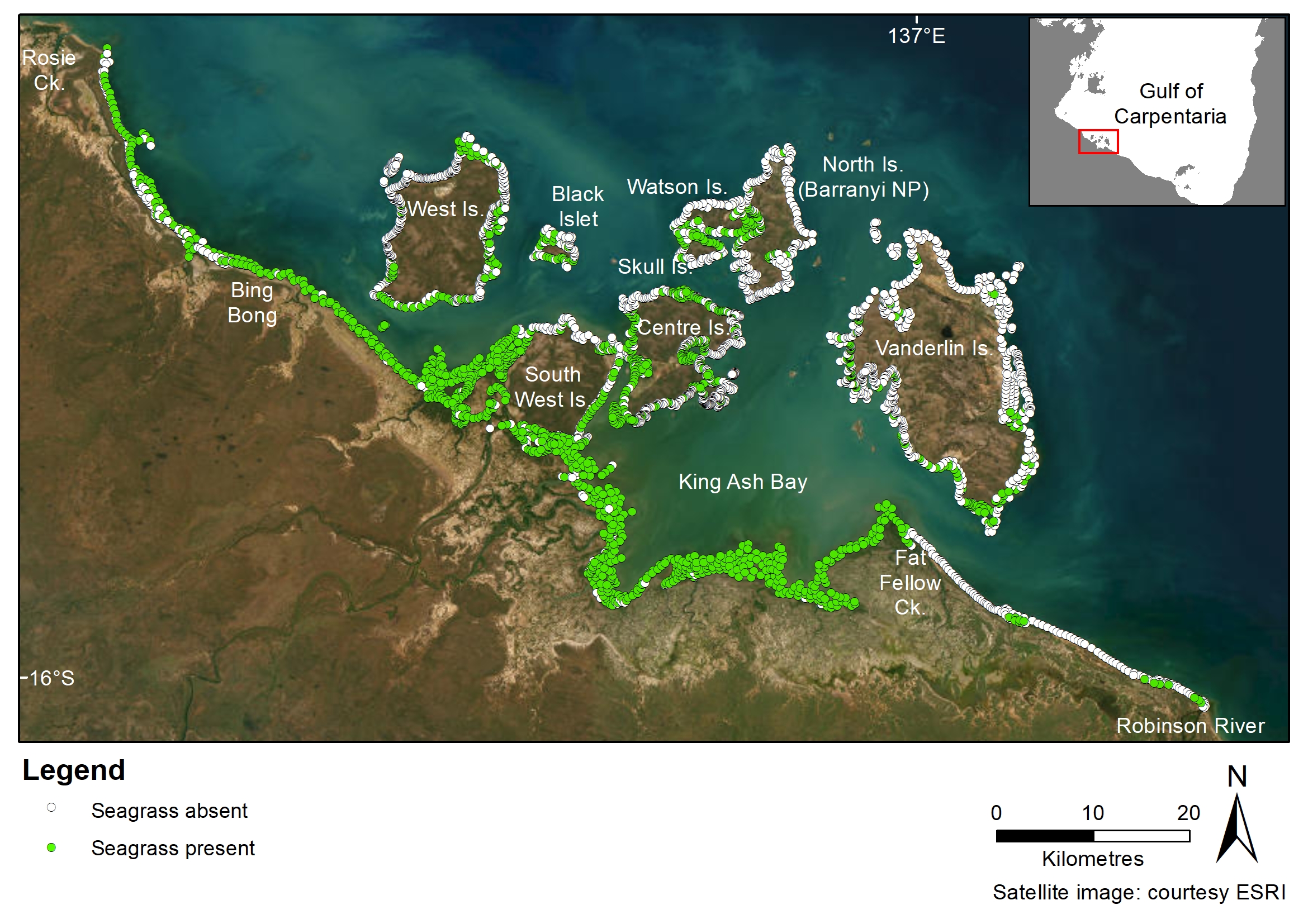
This dataset summarises benthic surveys in Yanyuwa Sea Country into 3 GIS shapefiles. (1) A point (site) shapefile describes seagrass presence/absence at 3248 sites surveyed by small vessel and helicopter. (2) The meadow shapefile describes attributes of 180 intertidal seagrass meadows. (3) The interpolation GeoTiff describes variation in seagrass biomass across the seagrass meadows. This project is a partnership between li-Anthawirriyarra rangers, Charles Darwin University, James Cook University, and Mabunji Aboriginal Resource Indigenous Corporation to map the intertidal habitats of the Yanyuwa Indigenous Protected Area (IPA), an area of profound importance to the Marra and Yanyuwa people and to the marine ecosystem of the Gulf of Carpentaria. Benthic habitat maps of Yanyuwa Country were produced, with a focus on seagrass. Report reference: Groom R, Carter A, Collier C, Firby L, Evans S, Barrett S, Hoffmann L, van de Wetering C, Shepherd L, Evans S, Anderson S. (2023) Mapping Critical Habitat in Yanyuwa Sea Country. Report to the National Environmental Science Program. Charles Darwin University, pp. 40. Available at: https://www.nespmarinecoastal.edu.au/wp-content/uploads/2023/07/NESP-MaC-Hub-Project-1.12_Groom-et-al-FINAL-REPORT.pdf Methods: The sampling methods used to study, describe and monitor seagrass meadows were developed by the TropWATER Seagrass Group and tailored to the location and habitat surveyed; these are described in detail in the relevant publications (https://research.jcu.edu.au/tropwater). Geographic Information System (GIS) All survey data were entered into a Geographic Information System (GIS) developed for Torres Strait using ArcGIS 10.8. Rectified colour satellite imagery of Yanyuwa Sea Country (Source: Allen Coral Atlas and ESRI), field notes and aerial photographs taken from the helicopter during surveys were used to identify geographical features, such as reef tops, channels and deep-water drop-offs, to assist in determining seagrass meadow boundaries. Three GIS layers were created to describe spatial features of the region: a site layer, seagrass meadow layer, and a seagrass biomass interpolation layer. Seagrass site layer This layer contains information on data collected at assessment sites. This layer includes: 1. Temporal survey details – Survey date; 2. Spatial position - Latitude/longitude; 3. Survey location; 4. Seagrass information including presence/absence of seagrass, above-ground biomass (total and for each species), percent cover of seagrass at each site and whether individual species were present/absent at a site; 5. Benthic macro-invertebrate information including the percent cover of hard coral, soft coral, sponges and other benthic macro invertebrates (e.g. ascidian, clam) at a site; 6. Algae information including percent cover of algae at a site and percent contribution of algae functional groups to algae cover at a site; 7. Open substrate – the percent cover of the site that had no flora or habitat forming benthic invertebrates present; 8. Dominant sediment type - Sediment type based on grain size visual assessment or deck descriptions. 9. Survey method and vessel 10. Relevant comments and presence/absence of megafauna and animals of interest (dugong, turtle, dolphin, evidence of dugong feeding trails); 11. Data custodians. Seagrass meadow layer Seagrass presence/absence site data, mapping sites, field notes, and satellite imagery were used to construct meadow boundaries in ArcGIS®. The meadow (polygon) layer provides summary information for all sites within each seagrass meadow, including: 1. Temporal survey details – Survey month and year as individual columns and the survey date (the date range the survey took place); 2. Spatial survey details – Survey location, meadow identification number that identifies the reef name and the meadow number. This allows individual meadows to be compared among years; 3. Survey method; 4. Meadow depth for subtidal meadows. Intertidal: meadow was mapped on an exposed bank during low tide; 5. Species presence – a list of the seagrass species in the meadow; 6. Meadow density – Seagrass meadows were classified as light, moderate, dense based on the mean biomass of the dominant species within the meadow. For example, a Thalassia hemprichii dominated meadow would be classed as “light” if the mean meadow biomass was <5 grams dry weight m-2 (g DW m-2), and “dense” if mean meadow biomass was >25 g DW m-2. 7. Meadow community type – Seagrass meadows were classified into community types according to seagrass species composition within each meadow. Species composition was based on the percent each species’ biomass contributed to mean meadow biomass. A standard nomenclature system was used to categorize each meadow. 8. Mean meadow biomass measured in g DW m-2 (+ standard error if available); 9. Meadow area (hectares; ha) (+ mapping precision) of each meadow was calculated in the GDA 2020 Geoscience Australia MGA Zone 53 projection using the ‘calculate geometry’ function in ArcMap. Mapping precision estimates (R; in ha) were based on the mapping method used for that meadow. Mapping precision estimate was used to calculate an error buffer around each meadow; the area of this buffer is expressed as a meadow reliability estimate (R) in hectares; 10. Any relevant comments; 11. Data custodians. Seagrass biomass interpolation layer An inverse distance weighted (IDW) interpolation was applied to seagrass site data to describe spatial variation in seagrass biomass within seagrass meadows. The interpolation was conducted in ArcMap 10.8. Base map The base map used is courtesy ESRI 2023. Format of the data: This dataset consists of 1 point layer package, 1 polygon layer package and 1 raster file: 1. Yanyuwa Sea Country sites 2021-2022.lpk - Symbology representing seagrass presence/absence at each survey site 2. Yanyuwa Sea Country seagrass meadows 2021-2022.lpk - Symbology representing dominant species (in terms of biomass) for each intertidal meadow. 3. Yanyuwa Sea Country seagrass biomass interpolation 2021-2022.lpk - Symbology representing the spatial variation in seagrass biomass within each seagrass meadow. Data dictionary: Yanyuwa Sea Country sites 2021-2022 (point data) SITE (text) - Unique identifier representing a single sample site MEADOW (text) - Unique identifier representing what meadow the sample site is located in. Blank if sample site is not located within a meadow SURVEY_DATE (numeric) – survey date (day/month/year) MONTH (text) – survey month YEAR (numeric) – survey year SURVEY_NAME (text) – Name of survey location LOCATION (text) – Name of survey location LATITUDE (numeric) – Site location in decimal degrees south LONGITUDE (numeric) – Site location in decimal degrees east TIME (numeric) – sample time (24 hours; GMT +9:30) (NT time - subtidal sites only) DEPTH (numeric) – depth recorded from vessel depth sounder (metres) for subtidal sites. Intertidal sites depth recorded as 0. DBMSL (numeric) – depth below mean sea level (metres) for subtidal sites. Intertidal sites depth recorded as 0. TIDAL (text) – identifying if the site was in an intertidal or subtidal location SUBSTRATE (text) – tags identifying the types of substrates at the sample site. Possible tags are Mud, Sand, Coarse Sand, Silt, Shell, Rock, Reef, Rubble and various combinations. Listed in order from most dominant substrate to least dominant. SEAGRASS_P (numeric) – Absence (0) or Presence (1) of seagrass SEAGRASS_C (numeric) - Estimated % of seagrass cover at sample site SEAGRASS_B (numeric) - Estimated total biomass per square metre for sample site calculated from the mean of three replicate quadrats. Unit is gdw m-2. SEAGRASS_SE (numeric) – standard error of biomass at sample site calculated from the three replicate quadrats used to estimate biomass at a sample site. Unit is gdw m-2. EXCLUDE_B (numeric) – Include (0) or Exclude (1). Any site identified that needs to be excluded from contributing to the calculation of mean meadow biomass, e.g. where a visual estimate of biomass could not be optioned (i.e. no visibility at the site, only a van Veen sediment grab was used at the site) C. rotundata (numeric) – Estimated biomass of Cymodocea rotundata at the sample site. Unit is gdw m-2. C. serrulata (numeric) – Estimated biomass of Cymodocea serrulata at the sample site. Unit is gdw m-2. E. acoroides (numeric) – Estimated biomass of Enhalus acoroides at the sample site. Unit is gdw m-2. H. uninervis (narrow) (numeric) – Estimated biomass of Halodule uninervis (narrow leaf morphology) at the sample site. Unit is gdw m-2. H. uninervis (wide) (numeric) – Estimated biomass of Halodule uninervis (wide leaf morphology) at the sample site. Unit is gdw m-2. H. decipiens (numeric) – Estimated biomass of Halophila decipiens at the sample site. Unit is gdw m-2. H. ovalis (numeric) – Estimated biomass of Halophila ovalis at the sample site. Unit is gdw m-2. H. spinulosa (numeric) – Estimated biomass of Halophila spinulosa at the sample site. Unit is gdw m-2. H. tricostata (numeric) – Estimated biomass of Halophila tricostata at the sample site. Unit is gdw m-2. S. isoetifolium (numeric) – Estimated biomass of Syringodium isoetifolium at the sample site. Unit is gdw m-2. T. ciliatum (numeric) – Estimated biomass of Thalassodendron ciliatum at the sample site. Unit is gdw m-2. T. hemprichii (numeric) – Estimated biomass of Thalassia hemprichii at the Z. muelleri (numeric) – Estimated biomass of Zostera muelleri at the sample site. Unit is gdw m-2. ALGAE_COVER (numeric) - Estimated % of algae cover at sample site (all algae types grouped) TURF_MAT (numeric) – (Turf mat algae % contribution to algae cover). Algae that forms a dense mat on the substrate ERECT_MACROPHYTE (numeric) – (Erect macrophyte algae % contribution to algae cover). Macrophytic algae with an erect growth form and high level of cellular differentiation, e.g. Sargassum, Caulerpa and Galaxaura species ENCRUSTING (numeric) – (Encrusting algae % contribution to algae cover). Algae that grows in sheet-like form attached to the substrate or benthos, e.g. coralline algae. ERECT_CALCAREOUS (numeric) – (Erect calcareous algae % contribution to algae cover). Algae with erect growth form and high level of cellular differentiation containing calcified segments, e.g. Halimeda species. FILAMENTOUS (numeric) – (Filamentous algae % contribution to algae cover). Thin, thread-like algae with little cellular differentiation. *Note: TURF_MAT + ERECT_MACROPHYTE + ENCRUSTING + ERECT_CALCAREOUS + FILAMENTOUS = 100% of algae cover HARD_CORAL (numeric) – (Hard coral %). All scleractinian corals including massive, branching, tabular, digitate and mushroom SOFT_CORAL (numeric) – (Soft coral %). All alcyonarian corals, i.e. corals lacking a hard limestone skeleton SPONGE (numeric) – (Sponge %) OTHER_BMI (numeric) – Any other benthic macro-invertebrates identified, e.g. oysters, ascidians, clams. Other benthic macro-invertebrates are listed in the “comments” attribute for intertidal and shallow subtidal camera drops, and listed as percent cover in the deepwater GIS. OPEN_SUBSTRATE (numeric) – Open substrate, no seagrass, algae or benthic macro-invertebrates at site DUGONG (numeric) - Absence (0) or Presence (1) of dugong/s at site TURTLE (numeric) - Absence (0) or Presence (1) of turtle/s at site DOLPHIN (numeric) - Absence (0) or Presence (1) of dolphin/s at site DFT PRESENT (numeric) - Absence (0) or Presence (1) of dugong feeding trails at site. Only clearly visible and therefore assessed at intertidal sites. Subtidal sites not assessed for DFTs coded as -999 METHOD (text) – e.g. helicopter, walking, hovercraft, boat-based including camera, free diving, scuba diving, van Veen grab, sled net VESSEL (text) – Vessel name (if known) COMMENTS (text) – Any comments for that site CUSTODIAN (text) – Custodian/owner of the data set UPDATED (text) - The date the shapefile was last updated AUTHOR (text) – Creator of GIS from the data set *Note: SEAGRASS_C + ALGAE_COVER + HARD_CORAL + SOFT_CORAL + SPONGE + OTHER_BMI + OPEN_SUBSTRATE = 100% of benthic cover Yanyuwa Sea Country seagrass meadows 2021-2022 (polygon data) ID (numeric) - Unique identifier representing a single meadow SURVEY_NAME (text) – Name of survey location LOCATION (text) – Name of survey location SURVEY_DATE (text) – Sample date (day/month/year) MONTH (numeric) – Sample month YEAR (numeric) – Sample year PERSISTENCE (text) – Meadow form on three categories: enduring, transitory, unknown DENSITY (text) – Meadow density categories (light, moderate, dense) TYPE (text) - Meadow community type determined according to seagrass species composition within the meadow SPECIES (text) – (Seagrass species): seagrass species found within the meadow. Species are recorded as abbreviated species names such as “E. acoroides” TOT_SITES (numeric) – (Number of survey sites): the number of sample sites within the meadow BIOMASS (numeric) – (Seagrass biomass (gdw m-2)): Mean biomass calculated from all sites (BIO_SITES) within an individual meadow SE (numeric) – (Standard Error (gdw m-2)): The error is a calculation of standard error of biomass from all (BIO_SITES) sites within an individual meadow. Where only 1 site surveyed in the meadow, SE will be 0. Where two sites were surveyed and biomass was 0 at one site, mean biomass and SE are the same values when calculated; AREA_HA (numeric) – (Meadow area (Ha)): Estimated meadow size (unit: hectares) R_M (numeric) – (Meadow mapping precision (m)): Estimated mapping precision based on mapping method. R_HA (numeric) - (Meadow reliability estimate (Ha)): Meadow reliability estimate (unit: hectares). Expressing the error buffer around each meadow as calculated from the mapping precision estimate SURVEY METHOD (text) – e.g. helicopter, walking, hovercraft, boat-based including camera, free diving, scuba diving, van Veen grab, sled net VESSEL (text) – Vessel name (if known) COMMENTS (text) – Any relevant comments for that meadow UPDATED (date) – The date the shapefile was last updated CUSTODIAN (text) – Custodian/owner of the data set AUTHOR (text) – Creator of GIS from the data set Yanyuwa biomass interpolation 2022 (interpolation layer) Inverse Distance Weighted interpolation. Band 1: Interpolated biomass in gdw m-2 Data Description: This section provides an brief text description of the data. This data set shows that in Yanyuwa sea country in the Gulf of Carpentaria, that there is significant seagrass along the coastline. The inshore coastline seagrass continues from Rosie Creek to Robinson River, where King Ash Bay and Bing Bong has almost continuous, reasonably dense seagrass meadows. Seagrass cover is present around the north, east and southern intertidal areas of West Island. Around the northern side of Black Islet has seagrass as well as north areas of Skull Island. Watson Island has seagrass areas on the southern and eastern coastlines. Seagrass cover can be found on Centre Island on all sides, particularly on the east and western sides. Vanderlin Island has light seagrass cover mostly towards the southern tip. Species present in these regions include C. serrulate, E. acoroides, H. ovalis, H. uninervis. eAtlas Processing: The original data were provided as ArcGIS Layer Packages (lpk]. Data were converted to Shapefiles and GeoTiff with no modifications to the underlying data. Location of the data: This dataset is filed in the eAtlas enduring data repository at: data\\custodian\NESP-MaC-1\1.12_Yanyuwa-sea-country-seagrass

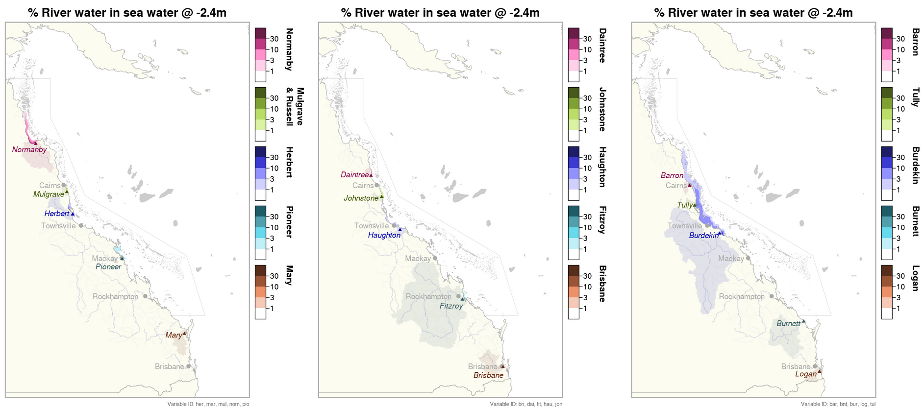
This generated data set contains summaries (daily, monthly) of the eReefs CSIRO river tracers model v2.0 (https://research.csiro.au/ereefs) outputs at 4km resolution, generated by the AIMS eReefs Platform (https://ereefs.aims.gov.au/ereefs-aims). These summaries are derived from the original daily model outputs available via the National Computing Infrastructure (NCI) (https://dapds00.nci.org.au/thredds/catalogs/fx3/catalog.html), and have been re-gridded from the original curvilinear grid used by the eReefs model into a regular grid so that the data files can be easily loaded into standard GIS software. These summaries are updated in near-real time daily and are made available via a THREDDS server (https://thredds.ereefs.aims.gov.au/thredds/ ) in NetCDF format. In addition to the variables containing single river data, we have added an 'all_rivers' variable which shows the total river water concentration (%) by combining all river output into a single variable. The eReefs river tracers model output contains passive river tracer results derived from version 2.0 of the 4km-resolution regional-scale hydrodynamic model of the Great Barrier Reef (GBR4). In the model, tracers are released at the river's mouth into its surface flow. These tracers move with the ocean currents, becoming more dilute as they spread out and mix with the ocean water, allowing the concentration of river water to be tracked over time. These tracers show the fraction of the water, at any given location, associated with each river. This model configuration and associated results dataset may be referred to as "GBR4_H2p0_Rivers" according to the eReefs simulation naming protocol. Description of the data: The data shows the percentage concentration of river water in the marine water. This is a good proxy for the extent of flood plumes associated with the major rivers along the Queensland coastline flowing into the Great Barrier Reef Marine Park. Flood plumes deliver sediments and nutrients into the ocean, both of which can result in detrimental effects on seagrass and reef habitats. Very low salinity concentrations in flood plumes can also cause bleaching and mortality on inshore reefs (this occurred during the flooding on Virago shoal off Townsville after the 2019 floods).This dataset represents only the concentration of river water in the marine environment. It does not model the changes in salinity, the nutrients levels or the sediment concentration in the water. These variables are calculated in the eReefs hydrodynamic model (salinity) and the biogeochemical model (nutrients and sediment). The river tracer is uniquely useful for tracing the origin of flood water back to the source river. The movement of the river water is driven by the surface ocean currents, that are driven largely by the wind. During most months the south easterly trade winds push the plumes back toward the coast in a northern direction. During the monsoon season, which is strongest between February and March, the winds drop and become more variable in direction. This means that flooding during these months is more variable in direction, occasionally moving southward and out to sea, sometimes reaching the mid shelf reefs. The width of the continental shelf narrows north of Townsville, resulting in it being easier for the flood plumes to reach the mid and outer reefs. Most significant flood plumes occur during the wet season from November to April. Flood plumes are less likely during the dry season from May to October. The plumes from some of the larger rivers can travel extensive distances during large flooding events. For example during 2019, flood waters from the Burdekin river travelled 700 km north along the coast, reaching Lizard Island. In 2017 the flood waters of the Fitzroy river reached the Whitsundays (450 km north) and the Normanby river water reached the tip of Cape York (440 km north). The rivers with the biggest discharge resulting in large flood plumes the Burdekin, Herbert, Tully, Johnstone, Russel, Mulgrave, Normanby, Fitzroy and Mary rivers. The following is a summary of the rivers with significant flood plumes during each year: 2015 Normanby, Mulgrave (minor), Johnstone (minor), Herbert (minor), Fitzroy, Mary 2016 Normanby, Mulgrave (minor), Tully (minor), Burdekin, Fitzroy, Mary (minor) 2017 Normanby, Johnstone, Herbert (minor), Tully (minor), Burdekin (major), Pioneer, Fitzroy (major), Burnett (minor), Mary (minor) 2018 Normanby, Mulgrave, Johnstone, Tully, Herbert, Burdekin, Mary (minor) 2019 Normanby, Daintree, Mulgrave, Johnstone, Tully, Herbert, Haugton (major), Burdekin (major), Pioneer (minor) 2020 Normanby (minor), Burdekin (minor), Fitzroy (minor) 2021 Normanby, Mulgrave (minor), Johnstone (minor), Tully (minor), Herbert, Burdekin (major), Fitzroy, Burnett (minor), Mary (minor) 2022 Normanby (minor), Daintree (minor), Mulgrave (minor), Johnstone (minor), Burdekin, Burnett (minor), Mary (major), Brisbane (minor), Logan (minor) 2023 Normanby, Herbert, Haugton (minor), Burdekin, Fitzroy (minor) Method: A description of the processing, especially aggregation and regridding, is available in the "Technical Guide to Derived Products from CSIRO eReefs Models" document (https://nextcloud.eatlas.org.au/apps/sharealias/a/aims-ereefs-platform-technical-guide-to-derived-products-from-csiro-ereefs-models-pdf). Data Dictionary: Variables: - nom: [% river water] Normanby - mul: [% river water] Mulgrave and Russell - jon: [% river water] Johnstone - her: [% river water] Herbert - bur: [% river water] Burdekin - fit: [% river water] Fitzroy - mar: [% river water] Mary - dai: [% river water] Daintree - bar: [% river water] Barron - tul: [% river water] Tully - hau: [% river water] Haughton - don: [% river water] Don - con: [% river water] O'Connell - pio: [% river water] Pioneer - bnt: [% river water] Burnett - fly: [% river water] Fly - cal: [% river water] Calliope - boy: [% river water] Boyne - cab: [% river water] Caboolture - log: [% river water] Logan - pin: [% river water] Pine - bri: [% river water] Brisbane - all_rivers: [% river water] Aggregation of all river outputs. This is a numerically addition of all single river variables to determine the total river water concentration (%). - time: [days since 1990-01-01 00:00:00 +10] Time - zc: [m] Z coordinate (depth) - depth slices - latitude: [degrees_north] Latitude (geographic projection) - longitude: [degrees_east] Longitude (geographic projection) Dimensions: - time - k (variable: zc) - latitude - longitude Depths: This data set contains the following depths, which are a subset of the depths available in the source data set [m]: -0.5, -1.5, -3.0, -5.55, -8.8, -12.75, -17.75, -23.75, -31.0, -39.5, -49.0, -60.0, -73.0, -88.0, -103.0, -120.0, -145.0. Limitations: This dataset is based on a spatial and temporal model and as such is an estimate of the environmental conditions. It is not based on in-water measurements. Furthermore, it should be noted that the river tracer product tracks the concentration of river water. It does not track sediment or nutrient in the water. As part of research into determining a suitable river concentration threshold for visualisations, we undertook many comparisons between the estimated flood plume extent from eReefs and those visible in Sentinel 2 satellite imagery. From this we found that the plume extent from eReefs was generally accurate to within about 10 km, with the most likely reason for the difference being slight errors in the model due to wind. The strength and direction of the wind is the predominant factor in determining the spread of the flood plumes. As a result any small errors in the modelling of the wind will lead to errors in the flood plume boundaries. The eReefs hydrodynamic model is driven by wind data from the Bureau of Meteorology's Access-R weather model, which is a forecast. It has a resolution of 12 km and so it is surprising that the eReefs model is as spatially accurate as it is. Part of the reason for this is that while the wind occasionally pushes the plumes offshore, the main determinant of the distribution is the dynamics of buoyant plumes. The rotation of the Earth acts to deflect to the left (in the Southern Hemisphere) any relative increase in motion between fluid layers. One such relative motion is a buoyant plume flowing over the top of denser ocean water. Deflected left on a river discharging along an east coast means it being pushed towards the coast. Thus, the plumes are trapped near the coast. The distance to which they spread from the coast is also set by this balance between density driven flow and the Earth’s rotation, something ocean models are very good at. The eReefs model tracks the percentage river water concentrations to very low levels, such as 1 part per million. At very low concentrations there is likely to not be ecologically relevant. When comparing the plume extents from the river tracer data with flood plumes visible in Sentinel 2 imagery we found that a concentration of 1% river water closely aligned with the visible edge of the flood plumes, where the water is darker and slightly green due to the increased levels of algae in the water.

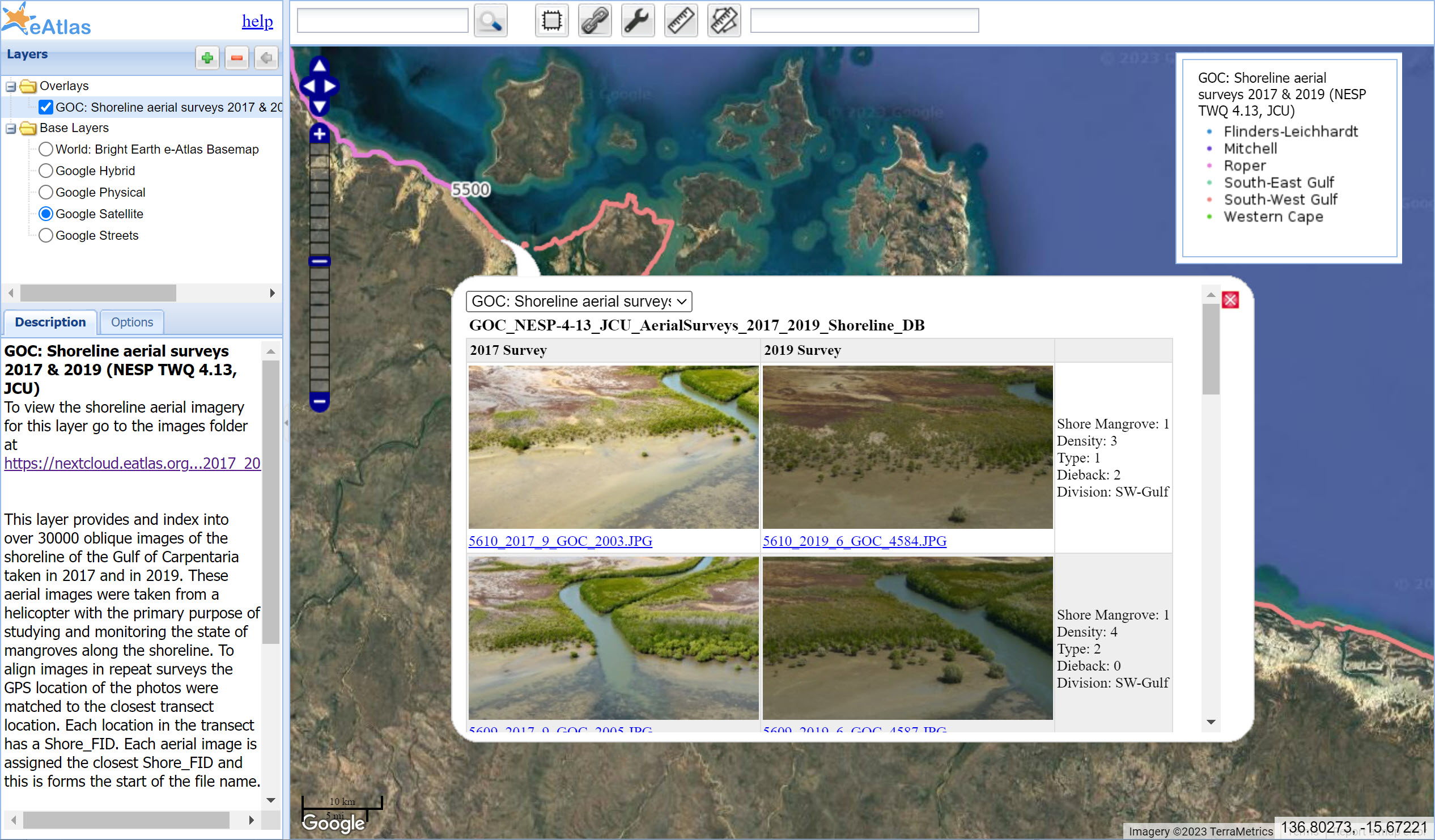
This project investigated the cause of the extensive areas of mangroves across the Gulf of Carpentaria which died in late 2015. Images from local fisherman showed extended impacted areas of more than 1,000 km where at least 7,400ha of mangroves had died in a matter of months. The project mapped the extent of the mass die-back, conducted aerial surveys to quantify shoreline condition, field studies to validate remote assessments and engaged with local aboriginal ranger groups to raise capacity for monitoring. The imagery can be viewed via a map interface https://maps.eatlas.org.au/index.html?intro=false&z=10&ll=136.96547,-15.79844&l0=ea_nesp4%3AGOC_NESP-4-13_JCU_AerialSurveys_2017_2019_Shoreline_DB,google_HYBRID or viewed as a gallery and downloaded in bulk https://nextcloud.eatlas.org.au/apps/sharealias/a/GOC_NESP-4-13_JCU_Mangrove-Shoreline-Aerial-Surveys_2017_2019 The aerial surveys are the first comprehensive record of oblique and continuous views of coastal shorelines for this large section of the Gulf of Carpentaria – providing a working database of more than 30,000 high-resolution images. This record is a lasting primary reference for baseline visual characterisations of shorelines for 2017 and 2019. The aim of aerial shoreline surveys was to systematically record and investigate the presence of 2015 mangrove dieback, the overall condition of shorelines, processes affecting the mangrove vegetation, and the health of tidal wetlands along Gulf shorelines, as well as in the mouths of major estuarine systems. These surveys were repeated in 2017 and in 2019 to gain insight and knowledge of the issues affecting shorelines, and the severity of factors influencing Gulf shorelines. The aerial surveys provided a baseline database or library of more than 19,534 geotagged oblique locations in 2017 and 2019 covering every metre of shoreline plus a series of inland profiles extending to the upper limits of tidal inundation in 37 estuarine outlets. This dataset consists of the complete set of imagery and compiled observations of current drivers of change and severity of impacts for 37 major estuarine sites. From east to west, these sites included Mission River, Embley River, Watson River, Holroyd River, Christmas Creek, Mitchell River, South Mitchell River, Nassau River, Staatan River, Gilbert River, Accident Inlet, Norman River, Flinders River, Leichhardt River, Albert River, Nicholson River, John’s Creek, Syrell Creek, Massacre Inlet, Dugong River, Toongoowahgun River, Elizabeth River, Sandalwood Place River, Calvert River, Robinson River, Wearyan River, McArthur River, Mule Creek, Limmen Bight River, Towns River, Roper River, Miyangkala Creek, Rose River, Muntak River, Walker River, and Koolatong River. (Note: we are still to publish the estuary survey data on the eAtlas). Shoreline and estuarine evaluations identified more than 30 issues in tidal wetland and shoreline habitats divided into direct and indirect human causes, or natural causes: shoreline retreat & landward transgressions of saline water and tidal wetland vegetation, rising sea levels, severe and frequent storms, feral animals plus other seemingly uncontrolled but damaging local land management practices. Methods: Aerial surveys were conducted in two series during 2017 and 2019. Those in 2017 were completed over 11 days from 1–11 December and included the shoreline survey plus surveys of 37 estuary mouths. The shoreline distance surveyed in 2017 was 2,633 km with a total flying distance of 4,646 km over 173 hours. A follow-up survey in 2019 was completed over nine days from 12–21 September and included the shoreline survey plus surveys of 31 estuary mouths. Aerial surveys were made using an R-44 helicopter flying at around 150 metres altitude. The aircraft windows and doors were removed to aid easier and best quality image capture. The entire shoreline from Mission River at Weipa (Queensland) to Koolatong River in Blue Mud Bay (Northern Territory) was surveyed. Shoreline and target estuaries were assessed in their order of occurrence travelling in a westerly direction. Shoreline filming captured the complete coastline used in the current evaluations of shoreline and estuarine habitat condition, with geotagged high-resolution digital images of shorelines, taken obliquely at low elevations ~150 metres altitude.. These photographs were comprised of three categories of images – survey, scenic and general. Survey photos made up ~60% and consisted of high-resolution images using a Nikon D800E camera with AF-S Nikkor 50 mm 1:1.4 G-series lens and di-GPS. These images were taken to give overlapping continuous coverage of shorelines centred up from the mean sea level contour – as the seaward edge of mangroves. Scenic photos made up ~33% and consisted of high resolution images using a Nikon D850 camera with AF-S Nikkor 28–300 mm 1:3.5–5.6 Gseries and di-GPS. A similar number and types of images were acquired in 2019. Summary of scenic photos: 2017 survey: Day 1: R44 Helicopter and crew on ground, jabiru in flight, crocodile on beach Day 2: Aerial view of mangrove die back, feral pigs on beach, jabiru in flight, large flock of egrets in mangrove forest Day 3: Aerial view of snubfin dolphin at surface, mangrove die back, smoke plume from bush fire in the distance creating a cloud, helicopter taking off. Day 4: Close up of rubber vine in a mangrove, pelican in flight, aerial image of swimming crocodile in turbid water with fish in its mouth, aerial shot of salt pans, crab pot on a mud flat. Day 5: Dead patch in mangrove forest due to lightning strike, aerial photos of mangrove die back, seagrass (long thin), aerial image of a dugong feeding trail through a seagrass meadow. Day 6: Indigenous coastal fish traps, sea eagle in flight, dugong stranded in mud, jabiru walking on sand, aerial photos of mangrove die back, shorebirds in flight Day 7: Dingy upside down on remote beach, aerial view of lush highly dense seagrass meadow (2 species, one with long leaves), dingy stranded in middle of mangrove forest, dark grey heron flying low over a river, fringing coral reef?, sea turtle, bent aero plane propeller partly covered in oysters, ghost net on shore Day 8: Large vertebra bone (whale?) on salt pan, turtle, helicopter in flight, aerial view of river mouth with seagrass meadows, Norm Duke standing in water holding seagrass Day 9: Large wrack of seagrass (tubular leaves), shore bird, mangrove die back, crocodile swimming with head out of water, boat ramp with two vehicles, industrial harbor, areas with large mangrove die back Day 10: Stranded dingy, aerial view of four green turtles, mangrove forest with large flock of black birds, ghost net caught up in mangrove, egret in flight over water, helicopter taking off from near mangrove, small town, aerial view of area with dense seagrass meadow Day 11: Closeup of water buffalo walking through water with long leafed seagrass, aerial view of 10 water buffalo, possibly indigenous fish traps, small town, river mouth with dense seagrass, large areas of mangrove die back 2019 survey: 0_sortedPhotos: images sorted by categories: Burdekin duck, crab pots, crocs, depositional gain, erosion, fire, inner fringe collapse, jabiru, jellies, large litter, light gaps, pelicans, root burial, shorebird Day 11: Ghost nets Day 12: Crocodile on mud flat, eight pelicans floating on water, pair of jabiru, collection of large tires on the shoreline presumably to help catch fish or crabs, samphire on a salt pan, helicopter in flight, crab pot at the edge of a mangrove, small boat wreckage on dry land at edge of mangrove, mangroves with fire in the distance, ghost nets on a beach, red dirt cliff where the shore is receding, weathered dead mangrove stumps, aerial shot crocodile swimming in clear water, aerial shot of wide sandy beach, two dead sharks on beach presumably caught and abandoned, jabiru in flight, flock of brolgas in flight, partly buried cage (protect turtle nest?) Day 13: tire and dog paw tracks on sandy beach with a dug up area (looking for turtle eggs?), black feral pig on beach, partly buried cage (to protect turtle nest?), blackened burnout grass neighbouring salt pan, pelican flying over water, dolphin and calf, person with fishing net on shore, small boat on water, photo of mangrove with a shadow of the helicopter on the water Day 14: giant milkweed growing on beach, grey mangrove saplings growing within trunks of dead mangrove trunks, flock of pelicans flying over water, old rotted mangrove tree stumps along the shoreline, mangrove forest with mixed species, many pig tracks on beach and rooting mounds, turtle tracks on beach, dust storm over salt flats, close up of shells on beach, many dead tree trunks on shoreline, dead trees covered in vines on shoreline, aerial view of wired fence going down beach into the intertidal region, three brolgas walking on beach, jabiru standing in a small lagoon near the shore, field of rotted mangrove tree stumps, large flock (> 30) of brolgas flying over mangroves and flats, brolgas on the shoreline at edge of grey mangrove forest, winding estuary lined with mangroves with large patches of die back, crocodile lying on muddy foreshore. Day 15 Both surveys were conducted during lower tidal levels where this was logistically feasible to do to gain the greatest visibility of the shoreline intertidal vegetation – positioned between the mean sea level and highest tide levels. Limitations of the data: The original aerial imagery data was reprocessed for presentation on the web. The the original aerial photos (which were 6144x4080 pixels) were down-sampled (3000x2000 pixels) and compressed (85% JPEG quality) to shrink the dataset size and make rapid previewing of the imagery much faster. This compression of the images reduced the total image dataset size from 310 GB down to 40 GB. The down-sampling resolution and compression level was chosen so that the images would retain nearly all the visual information of the original images. To allow researchers to assess whether this compression has lost key visual information, a folder on the download page (original-vs-compressed) contains a representative sample of both the original photos and their compress form is available. The original, full resolution versions of the photos is not available for direct download, but can be requested by contacting the eAtlas team via e-atlas@aims.gov.au, noting that to obtain the full dataset we would need to transfer the dataset using a hard drive. Format of the data: - Shoreline Aerial imagery: Georeferenced JPEG images (6144x4080 pixels), labelled with a Shore_FID that cross references into the Shoreline Database (Original Excel spreadsheet NESP_GOC_AerialSurveys_2017_2019.xlsx, or processed GOC_NESP-4-13_JCU_AerialSurveys_2017_2019_Shoreline_DB.shp Shapefile). The 2017 survey contains 16,706 images. The 2019 survey contains 17,161 images. Note: Only download-sampled (3000x2000 pixels) versions of this imagery are available directly through the eAtlas. - Scenic imagery: 2017: 354 JPEG files in 13 folders. 2019: 502 JPEG files in 15 folders. Note: The eAtlas makes available the original scenic images without recompression. Data dictionary: NESP_GOC_AerialSurveys_2017_2019.xlsx: TAB: Shoreline_Image_Database_17_19 - Shore_FID: Identifier of the segment along the shoreline transect. This is a continuous counter from 1 (North West of Gulf of Carpentaria) to 19534 (Western side of Cape York). Each segment is space approxiately 100 m apart. Images in the survey are aligned to the closest transect segment. This allows the repeat surveys over multiple years to be compared. - Shore_X: Longitude of the shoreline transect location. - Shore_Y: Latitude of the shoreline transect location. - Folder_2017: Path of the original imagery. This is not very useful when the data is moved. - 2017_Image: Filename of the photo from the 2017 survey. For example: 19533_2017_1_GOC_7213.JPG - Folder_2019: Path of the original imagery. This is not very useful when the data is moved. - 2019_Image: Filename of the photo from the 2019 survey. For example: 19533_2019_1_GOC_2864.JPG - 2017_Hyperlink: Link to images on disk (only works if the imagery is saved in the sample location as the original storage) - 2019_Hyperlink: Link to images on disk (only works if the imagery is saved in the sample location as the original storage) TAB: Shoreline_Observations WAYPOINT (#) - Latitude - Longitude - Date - Created - Turtle - Turtle_Track - Croc - Pig_Track - Vehicles - Net - Large_Litter - Small_Litter - Crab_Pot - Abandoned_Crab_Pot - Set_Net - Cattle_Track - Dead_Turtle - Turtle_Nest - SHARK - EAGLE_RAY - RAY - Rope - Dolphin - Dugong - Pig_Digging - Abandoned_Boat - Shorebird_Roost - SHOVELNOSE - DEAD_RAY - SAWFISH - DINGO - CURLEW - MANTA NESP_GOC_AerialSurveys_2017_2019.xlsx: TAB: Shore_DieBack_MAP - Shore_FID: ID of the location along the shoreline transect. - Image_ID_2017: Filename of the image from 2017 survey, prior to having the Shore_ID prepended to it. - Image_ID_2019: Filename of the image from 2019 survey, prior to having the Shore_ID prepended to it. - X_2017 - X_2019 - Shore_Mangrove - Density - Type - Dieback GOC_NESP-4-13_JCU_AerialSurveys_2017_2019_Shoreline_DB.shp This is a conversion of some of the information from NESP_GOC_AerialSurveys_2017_2019.xlsx into a shapefile suitable for mapping. Details of this conversion is detailed at https://github.com/eatlas/GOC_JCU_NESP-TWQ-4-13_Mangrove-Dieback_2017-2019. - Shore_FID: Shore_FID. Identifier of the segment along the shoreline transect. This is a continuous counter from 1 (North West of Gulf of Carpentaria) to 19534 (Western side of Cape York). Each segment is spaced approxiately 100 m apart. Images in the survey are aligned to the closest transect segment. This allows the repeat surveys over multiple years to be compared. - Image_ID_2017: ImgID_2017. Name of the original 2017 aerial photograph, prior to adding the Shore_FID to the image filename. - Image_ID_2019: ImgID_2019. Name of the original 2019 aerial photograph, prior to adding the Shore_FID to the image filename. - X_2017:** X_2017. ?? - X_2019:** X_2019. ?? - Shore_Mangrove: Shore_Mang. - Density: Density. - Type: Type. - Dieback: Dieback. - ImageCount: Number of survey images in each transect segment. 0 - No survey imagery, 1 - One image from either 2017 or 2019, 2 - images from both 2017 and 2019. - Division: Division of the shoreline into sections correspond to major river catchments. The Division attribute is the human readable version of the division name. - DivShort: Short version of the division name. This is used for the directories that the images are stored in. Having the images split into these regions limits the number of images per directory and allows users to download a division subsection of the imagery. - Division (DivShort) - Roper (Roper) - South-West Gulf (SW-Gulf) - Flinders-Leichhardt (FL-group) - South-East Gulf (SE-Gulf) - Mitchell (Mitchell) - Western Cape (W-Cape) eAtlas Processing: The original data was reprocessed for presentation on the web. This included down-sampling (3000x2000 pixels) and recompressing (85% JPEG quality) the original aerial photos (which were 6144x4080 pixels) so that the total image dataset size was reduced from 310 GB down to 40 GB. The down-sampling and compression was chosen so that the images retain nearly all the visual information of the original images. To allow researchers to assess whether this compression has lost key visual information a folder (original-vs-compressed) containing a representative sample of both the original photos and their compress form is available. The original, full resolution versions of the photos is not available for download, but can be requested by contacting the eAtlas team via e-atlas@aims.gov.au. Location of the data: This dataset is filed in the eAtlas enduring data repository at: data\\custodian\2018-2021-NESP-TWQ-4\4.13_Assessing-gulf-mangrove-dieback Publications: A. Existential projects ::: Independent seagrass surveys in the GOC Carter, A., S. McKenna, M. Rasheed, H. Taylor, C. v. d. Wetering, K. Chartrand, C. Reason, C. Collier, L. Shepherd, J. Mellors, L. McKenzie, N.C. Duke, A. Roelofs, N. Smit, R. Groom, D. Barrett, S. Evans, R. Pitcher, N. Murphy, M. Carlisle, M. David, S. Lui, T. S. I. Rangers and R. Coles. 2023. Seagrass spatial data synthesis from north-east Australia, Torres Strait and Gulf of Carpentaria, 1983 to 2022. Limnology and Oceanography published online: 16 pp. https://doi.org/10.1002/lol2.10352 Independent evaluations of climate conditions regards the GOC mangrove dieback event Chung, C.T.Y., P. Hope, L.B. Hutley, J. Brown and N.C. Duke. 2023. Future climate change will increase risk to mangrove health in Northern Australia. Communications Earth & Environment 4, Article 192. 8 pages. https://doi.org/10.1038/s43247-023-00852-z Abhik, S., P. Hope, H. H. Hendon, L. B. Hutley, S. Johnson, W. Drosdowsky, J. R. Brown and N. C. Duke. 2021. Influence of the 2015-16 El Niño on the record-breaking mangrove dieback along northern Australia coast. Scientific Reports 11(20411): 12 pp. https://doi.org/10.1038/s41598-021-99313-w Harris, T., P. Hope, E. Oliver, R. Smalley, J. Arblaster, N. Holbrook, N. Duke, K. Pearce, K. Braganza and N. Bindoff. 2017. Climate drivers of the 2015 Gulf of Carpentaria mangrove dieback. Australia, NESP Earth Systems and Climate Change Hub: 31 pages. JCU TropWATER Report #17/57. Independent assessment of mangrove plant physiological conditions regards the GOC mangrove dieback event Gauthey, A., D. Backes, J. Balland, I. Alam, D.T. Maher, L.A. Cernusak, N.C. Duke, B.E. Medlyn, D. T. Tissue and B. Choat. 2022. Natural water-availability gradient accentuates the risk of hydraulic failure in Avicennia marina during physiological drought. Frontiers Plant Science 13: 822136. https://doi.org/10.3389/fpls.2022.822136 Independent evaluation of marine fisheries debris observed along GOC shorelines Hardesty, B. D., L. Roman, N. C. Duke, J.R. Mackenzie and C. Wilcox. 2021. Abandoned, lost and derelict fishing gear ‘ghost nets’ are increasing through time. Marine Pollution Bulletin 173 (112959): 10pp. https://doi.org/10.1016/j.marpolbul.2021.112959 Independent evaluation with global examples of ecosystem decline includes the mass dieback of GOC mangroves Bergstrom, D. M., B. C. Wienecke, J. van der Hoff, L. Hughes, D. L. Lindemayer, T. D. Ainsworth, C. M. Baker, L. Bland, D. M. J. S. Bowman, S. T. Brooks, J. G. Canadell, A. Constable, K. A. Dafforn, M. H. Depledge, C. R. Dickson, N. C. Duke, K. J. Helmstedt, C. R. Johnson, M. A. McGeoch, J. Melbourne-Thomas, R. Morgain, E. N. Nicholson, S. M. Prober, B. Raymond, E. G. Ritchie, S. A. Robinson, K. X. Ruthrof, S. A. Setterfield, C. M. Sgro, J. S. Stark, T. Travers, R. Trebilco, D. F. L. Ward, G. M. Wardle, K. J. Williams, P. J. Zylstra and J. D. Shaw. 2021. Ecosystem collapse from the tropics to the Antarctic: an assessment and response framework. Global Change Biology 27: 1692-1703. https://doi.org/10.1111/gcb.15539 Harris, R. M., L. J. Beaumont, T. Vance, C. Tozer, T. A. Remenyi, S. E. Perkins-Kirkpatrick, P. J. Mitchell, A. B. Nicotra, S. McGregor, N. R. Andrew, M. Letnic, M. R. Kearney, T. Wernberg, L. B. Hutley, L. E. Chambers, M. Fletcher, M. R. Keatley, C. A. Woodward, G. Williamson, N.C. Duke and D. M. Bowman 2018. Linking climate change, extreme events and biological impacts. Nature Climate Change 8(7): 579-587. DOI: 10.1038/s41558-018-0187-9. Author Correction: Nature Climate Change 8(9): 1; DOI: 10.1038/s41558-018-0237-3. B. NESP project reporting ::: Duke, N.C., J.R. Mackenzie, A.D. Canning, L.B. Hutley, A.J. Bourke, J.M. Kovacs, R. Cormier, G. Staben, L. Lymburner and E. Ai. 2022. ENSO-driven extreme oscillations in mean sea level destabilise critical shoreline mangroves – an emerging threat with greenhouse warming. PLOS Climate 1(8), 23pp. https://doi.org/10.1371/journal.pclm.0000037. Duke, N.C. 2022. Climate change killed 40 million Australian mangroves in 2015. Here’s why they’ll probably never grow back. The Conversation: online. 28 July 2022. https://theconversation.com/climate-change-killed-40-million-australian-mangroves-in-2015-heres-why-theyll-probably-never-grow-back-166971 Duke, N.C., L.B. Hutley, J.R. Mackenzie, D. Burrows. 2021. Processes and factors driving change in mangrove forests – an evaluation based on the mass dieback event in Australia’s Gulf of Carpentaria. In: ‘Ecosystem Collapse - and Climate Change’, editors: Josep G. Canadell and Robert B. Jackson, Springer, Ecol. Studies 241: 221-264. https://link.springer.com/chapter/10.1007/978-3-030-71330-0_9 Duke, N.C., Mackenzie, J., Kovacs, J., Staben, G., Coles, R., Wood, A., & Castle, Y. 2020. Assessing the Gulf of Carpentaria mangrove dieback 2017–2019. Volume 1: Aerial surveys. Report to the National Environmental Science Program. James Cook University, Townsville, 226 pp. https://nesptropical.edu.au/wp-content/uploads/2021/05/Project-4.13-Final-Report-Volume-1.pdf Duke, N.C., Mackenzie, J., Hutley, L., Staben, G., & Bourke, A. 2020. Assessing the Gulf of Carpentaria mangrove dieback 2017–2019. Volume 2: Field studies. Report to the National Environmental Science Program. James Cook University, Townsville, 150 pp. https://nesptropical.edu.au/wp-content/uploads/2021/ 05/Project-4.13-Final-Report-Volume-2.pdf Duke, N.C. 2020. Mangrove harbingers of coastal degradation seen in their responses to global climate change coupled with ever-increasing human pressures. Human Ecology Journal of the Commonwealth Human Ecology Council – Mangrove Special Issue 30: 19-23. https://www.checinternational.org/wp-content/uploads/2020/06/Journal-30-Mangroves.pdf Duke, N.C., C. Field, J.R. Mackenzie, J.-O. Meynecke and A.L. Wood. 2019. Rainfall and its possible hysteresis effect on the proportional cover of tropical tidal wetland mangroves and saltmarsh-saltpans. Marine and Freshwater Research 70(8): 1047-1055. DOI: 10.1071/MF18321. Van Oosterzee, Penny, and Duke, Norman 2017. Extreme weather likely behind worst recorded mangrove dieback in northern Australia. The Conversation, 14 March 2017, online. pp. 1-6. http://theconversation.com/extreme-weather-likely-behind-worst-recorded-mangrove-dieback-in-northern-australia-71880 Duke, N. C., J. M. Kovacs, A. D. Griffiths, L. Preece, D. J. E. Hill, P. v. Oosterzee, J. Mackenzie, H. S. Morning and D. Burrows. 2017. Large-scale dieback of mangroves in Australia’s Gulf of Carpentaria: a severe ecosystem response, coincidental with an unusually extreme weather event. Marine and Freshwater Research 68 (10): 1816-1829. http://dx.doi.org/10.1071/MF16322 Duke, N.C. 2017. Climate calamity along Australia's gulf coast. Landscape Architecture Australia 153: 66-71. https://landscapeaustralia.com/articles/february-issue-of-laa-out-now-1/# Duke, N. C. 2016. Huge mangrove die-off in Australia. Nature 535: 204. http://dx.doi.org/10.1038/535204a Duke, N.C. 2021. Assessing mangrove dieback in the Gulf of Carpentaria. National Environmental Science Program, Northern Australia Environmental Resources and Tropical Water Quality Hubs, Wrap-up factsheet, 6 pages. https://nesptropical.edu.au/wp-content/uploads/2021/05/Project-4.13-Wrap-up-Factsheet.pdf Duke, N.C. 2021. Facilitating natural regeneration processes: Planting seedlings is not the best response to mass mangrove dieback in the Gulf of Carpentaria. Report to the National Environmental Science Program. Reef and Rainforest Research Centre Limited, Cairns, 8 pages. https://nesptropical.edu.au/wp-content/uploads/2021/08/Project-6.2-Case-Study-Booklet-1-Mangroves_COMPLETE_FINAL2.pdf Duke, N.C., Mackenzie, J. 2020. Assessing the Gulf of Carpentaria mangrove dieback 2017–2019: Summary report. James Cook University, Townsville (41pp.). 55 pages. https://nesptropical.edu.au/wp-content/uploads/2021/05/Project-4.13-Summary-Report.pdf Duke, N.C. 2020. Assessing mangrove dieback in the Gulf. National Environmental Science Program, Northern Australia Environmental Resources Hub, Start-up factsheet, 4 pages. https://nesptropical.edu.au/wp-content/uploads/2020/01/Mangrove-dieback-start-up-factsheet_NAER.pdf Duke, N.C. 2019. Assessing mangrove dieback in the Gulf of Carpentaria. National Environmental Science Program, Northern Australia Environmental Resources Hub, Project Update June 2019, 2 pages. https://nesptropical.edu.au/wp-content/uploads/2020/01/Mangrove-dieback-update-June-2019-1_NAER.pdf Duke, N.C. 2019. Assessing the Gulf of Carpentaria mangrove dieback. National Environmental Science Program, Tropical Water Quality Hub, Factsheet, 2 pages. https://nesptropical.edu.au/wp-content/uploads/2019/04/NESP-TWQ-Project-4.13-Factsheet.pdf

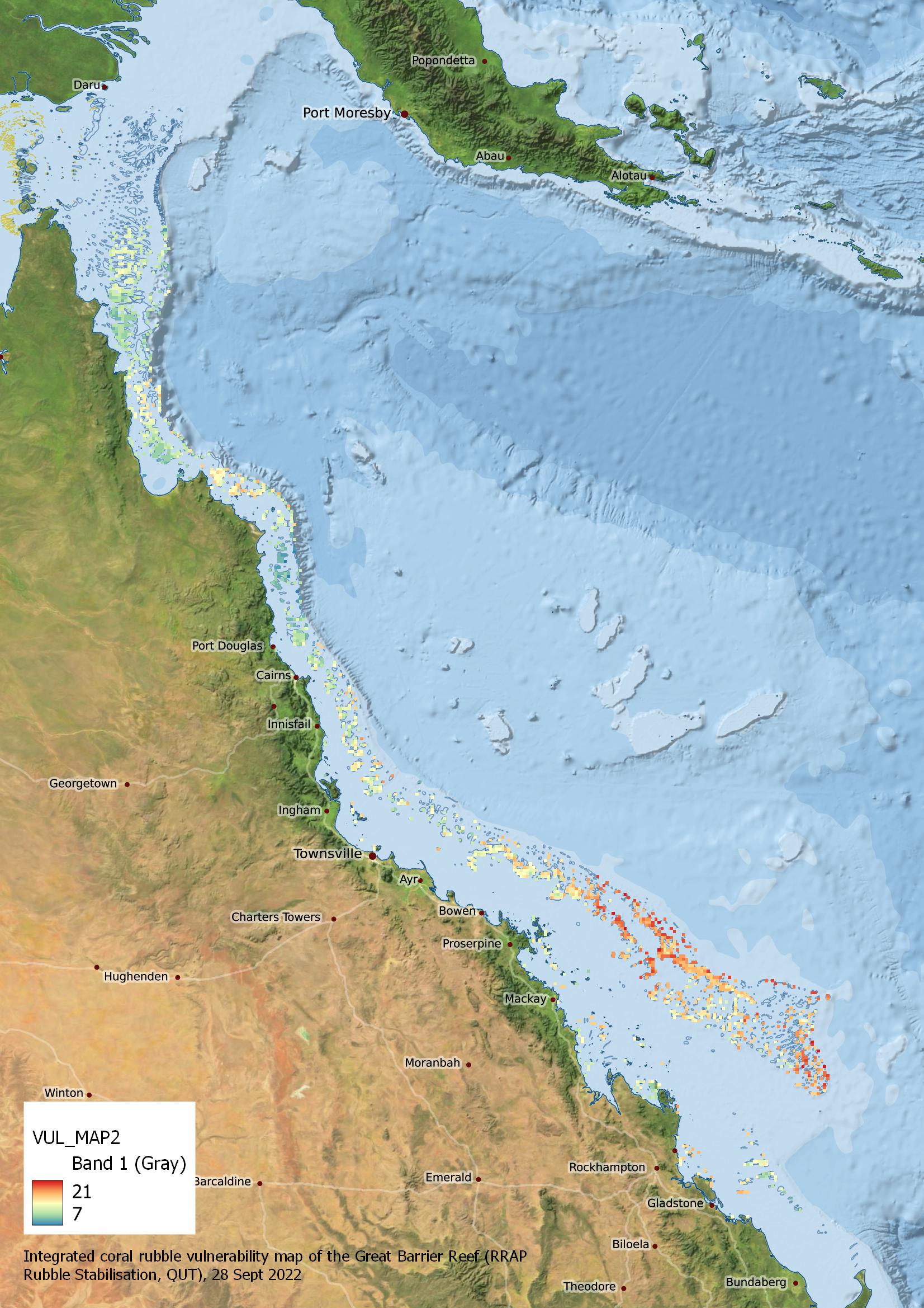
This vulnerability map results from integrating the spatial pattern of the following stressors: cyclonic waves, currents, cyclone tracks, heatwaves (DHW), crown of thorns starfish, and tsunamis. After summarizing historical data and reclassifying each variable into a common scale, they were integrated into a single vulnerability score whose spatial distribution is represented in this map. Methods The coral rubble vulnerability map was calculated by combining GBR wide datasets on currents (2015-2019), cyclone wave statistics (synthetic cyclones), Degree Heating Weeks (DHW) (1986-2021), crown of thorns starfish outbreaks (1985-2017), cyclone tracks (1950-2022), and tsunamis hazard (Probabilistic Tsunami Hazard Assessment, PTHA18). Each of these datasets were converted onto a common 0.005° raster grid (matching the final vulnerability map) using inverse distance weighting (IDW) interpolation for point format datasets (cyclone track points, COTs, tsunamis) and resampling (currents) for raster datasets. For wave and DHW the data was reprojected and resampled on to the common grid. These grids were then clipped to the GBRMPA GBR features reef boundaries. In order to obtain the vulnerability score, each variable was reclassified in ArcGIS Pro, using five equally spaced categories (quantising the data into discrete levels between the minimum and maximum values). As result, all variables ranged from 1 to 5. Finally, all six layers were added up, ignoring no-data pixels. In the case of currents, cyclonic waves and DHW, multiple measures were reviewed and considered. In the index maximum surface current, maximum significant wave height from cyclones and mean DHW were used. Further details of the input data can be found in the ‘Supplementary information - Maps of input data for integrated coral rubble vulnerability map of the Great Barrier Reef’. Limitations This first vulnerability map assumes equal weight for all variables included. There is an ongoing study aiming to test and identify which variables are more correlated with reef damage. This model does not consider the likely accumulation of rubble based on the topology of the reefs. It does not consider the production rate of coral that can result in coral rubble or that some of the inshore reefs particularly in Broad Sound are not coral reefs. Format The spatial model is 1988x2707 pixels with a spatial reference of WGS84 (EPSG:2346). The original dataset is stored in ESRI GRID format (6322 KB), which was converted to a GeoTiff for use in the eAtlas (22 MB). Data dictionary Pixel values in the raster correspond to low vulnerability (7) through to high vulnerability (23)

This dataset details the Declared Indigenous Protected Areas (IPA) across Australia through the implementation of the Indigenous Protected Areas Programme. These boundaries are not legally binding. An Indigenous Protected Area (IPA) is an area of Indigenous-owned land or sea where traditional Indigenous owners have entered into an agreement with the Australian Government to promote biodiversity and cultural resource conservation. The Indigenous Protected Areas element of the Caring for our Country initiative supports Indigenous communities to manage their land as IPAs, contributing to the National Reserve System. Further information can be found at the website below. http://www.environment.gov.au/indigenous/ipa/index.html Declared IPAs in order of gazettal date: Nantawarrina Preminghana Risdon Cove putalina Deen Maar Yalata Warul Kawa Watarru Walalkara Mount Chappell Island Badger Island Dhimurru Guanaba Wattleridge Mount Willoughby Paruku Ngaanyatjarra Tyrendarra Toogimbie Anindilyakwa Laynhapuy - Stage 1 Ninghan North Tanami Warlu Jilajaa Jumu Kaanju Ngaachi Great Dog Island Babel Island lungatalanana Angas Downs Pulu Islet Tarriwa Kurrukun Warddeken Djelk Jamba Dhandan Duringala Kurtonitj Framlingham Forest Kalka - Pipalyatjara Boorabee and The Willows Lake Condah Marri-Jabin (Thamurrurr - Stage 1) Brewarrina Ngemba Billabong Uunguu - Stage 1 Apara - Makiri - Punti Antara - Sandy Bore Dorodong Weilmoringle Yanyuwa (Barni - Wardimantha Awara) Minyumai Gumma Mandingalbay Yidinji Southern Tanami Angkum - Stage 1 Ngunya Jargoon Birriliburu Eastern Kuku Yalanji Bardi Jawi Girringun Wilinggin Dambimangari Balanggarra Thuwathu/Bujimulla Yappala Wardaman - Stage 1 Karajarri - Stage 1 Nijinda Durlga - Stage 1 Note: This record is a copy from the Department of the Environment for use in the eAtlas. For the latest version of this dataset check the Department of the Environment website.

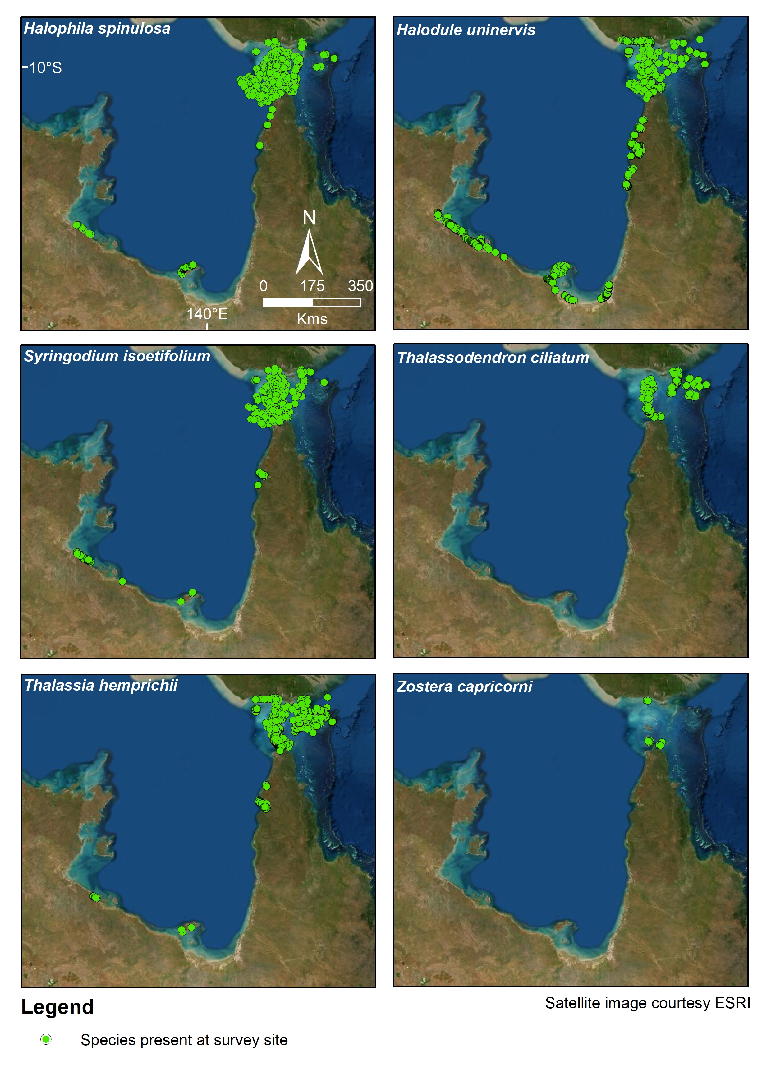
This dataset summarises 40 years of seagrass data collection (1983-2022) within Torres Strait and the Gulf of Carpentaria into two GIS shapefiles: (1) a point shapefile that includes survey data for 48,612 geolocated sites, and (2) a polygon geopackage describing seagrass at 641 individual or composite meadows. Managing seagrass resources in northern Australia requires adequate baseline information on where seagrass is (presence/absence), the mapped extent of meadows, what species are present, and date of collection. This baseline is particularly important as a reference point against which to compare seagrass loss or change through time. The scale of northern Australia and the remoteness of many seagrass meadows from human populations present a challenge for research and management agencies reporting on the state of seagrass ecological indicators. Broad-scale and repeated surveys/studies of areas are logistically and financially impractical. However seagrass data is being collected through various projects which, although designed for specific reasons, are amenable to collating a picture of the extent and state of the seagrass resource. In this project we compiled seagrass spatial data collected during surveys in Torres Strait and the Gulf of Carpentaria into a standardised form with point-specific and meadow-specific spatial and temporal information. We revisited, evaluated, simplified, standardised, and corrected individual records, including those collected several decades ago by drawing on the knowledge of one of our authors (RG Coles) who led the early seagrass data collection and mapping programs. We also incorporate new data, such as from photo records of an aerial assessment of mangroves in the Gulf of Carpentaria in 2017. This project was funded by the National Environmental Science Programme (NESP) Marine and Coastal Hub and Torres Strait Regional Authority (TSRA) in partnership with the Centre for Tropical Water and Aquatic Ecosystem Research (TropWATER), James Cook University. The project follows on from TropWATER’s previous work compiling 35 years of seagrass spatial point data and 30 years of seagrass meadow extent data for the Great Barrier Reef World Heritage Area (GBRWHA) and adjacent estuaries, funded through successive NESP Tropical Water Quality Hub Projects 3.1 (2015-2016) and 5.4 (2018-2020). These data sets are now publicly available through the eAtlas data portal: https://doi.org/10.25909/y1yk-9w85 . In making this data publicly available for management, the authors and data custodians request being contacted and involved in decision making processes that incorporate this data, to ensure its limitations are fully understood. Methods: The data were collected using a variety of survey methods to describe and monitor seagrass sites and meadows. For intertidal sites/meadows, these include walking, observations from helicopters in low hover, and observations from hovercraft when intertidal banks were exposed. For subtidal sites/meadows, methods included free diving, scuba diving, video transects from towed cameras attached to a sled with/without a sled net, video drops with filmed quadrats, trawl and net samples, and van Veen grab samples. These methods were selected and tailored by the data custodians to the location, habitat surveyed, and technology available. Important site and method descriptions and contextual information is contained in the original trip reports and publications for each data set provided in Table 1 of Carter et al. (2022). Geographic Information System (GIS) Mapping data for historic records (1980s) were transcribed from original logged and mapped data based on coastal topography, dead reckoning fixes and RADAR estimations. More recent data (1990’s onwards) is GPS located. All spatial data were converted to shapefiles with the same coordinate system (GDA 1994 Geoscience Australia Lambert), then compiled into a single point shapefile and a single polygon shapefile (seagrass meadows) using ArcMap (ArcGIS version 10.8 Redlands, CA: Environmental Systems Research Institute, ESRI). Some early spatial data was offset by several hundred metres and where this occurred data was repositioned to match the current coastline projection. The satellite base map used throughout this report is courtesy ESRI 2022. Seagrass Site Layer: This layer contains information on data collected at assessment sites, and includes: 1. Temporal survey details – Survey month and year; 2. Spatial position - Latitude/longitude; 3. Survey name; 4. Depth for each subtidal site is m below MSL Depth and was extracted from the Australian Bathymetry and Topography Grid, June 2009 (Whiteway 2009). This approach was taken due to inconsistencies in depth recordings among data sets, e.g., converted to depth below mean sea level, direct readings from depth sounder with no conversion, or no depth recorded. Depth for intertidal sites was recorded as 0 m MSL, with an intertidal site defined as one surveyed by helicopter, walking, or hovercraft when banks were exposed during low tide; 5. Seagrass information including presence/absence of seagrass, and whether individual species were present/absent at a site; 6. Dominant sediment - Sediment type in the original data sets were based on grain size analysis or deck descriptions. For consistency, in this compilation we include only the most dominant sediment type (mud, sand, shell, rock, rubble), removed descriptors such as “fine”, “very fine”, “coarse”, etc., and replaced redundant terms, e.g. “mud” and “silt” are termed “mud”; 7. Survey methods – In this compilation we have updated and standardised the terms used to describe survey methods from the original reports; and 8. Data custodians. Seagrass Meadow Layer: Polygons in the meadow layer are drawn from extent data collected during some surveys. Not all surveys collected meadow extent data (e.g., Torres Strait lobster surveys). The seagrass meadow layer is a composite of all the spatial polygon data we could access where meadow boundaries were mapped as part of the survey. All spatial layers were compiled into a single spatial layer using the ArcToolbox ‘merge’ function in ArcMap. Where the same meadow was surveyed multiple times as part of a long-term monitoring program, the overlapping polygons were compiled into a single polygon using the ‘merge’ function in ArcMap. Because meadows surveyed more than once were merged, there were some cases where adjacent polygons overlap each other. Meadow Data Includes: 1. Temporal survey details – Survey month and year, or a list of survey dates for meadows repeatedly sampled; 2. Survey methods; 3. Meadow persistence – Classified into three categories: a. Unknown – Unknown persistence as the meadow was surveyed less than five times; b. Enduring – Seagrass is present in the meadow ≥90% of the surveys; c. Transitory – Seagrass is present in the meadow <90% of the surveys; 4. Meadow depth – Classified into three categories: a. Intertidal – Meadow was mapped on an exposed bank during low tide, e.g. Karumba monitoring meadow; b. Subtidal – Meadow remains completely submerged during spring low tides, e.g. Dugong Sanctuary meadow; c. Intertidal-Subtidal – Meadow includes sections that expose during low tide and sections that remain completely submerged, e.g. meadows adjacent to the Thursday Island shipping channel; 5. Dominant species of the meadow based on the most recent survey; 6. Presence or absence of individual seagrass species in a meadow; 7. Meadow density categories – Seagrass meadows were classified as light, moderate, dense, variable or unknown based on the consistency of mean above-ground biomass of the dominant species among all surveys, or percent cover of all species combined (see Table 2 in Carter et al. 2022). For example, a Halophila ovalis dominated meadow would be classed as “light” if the mean meadow biomass was always <1 gram dry weight m-2 (g DW m-2) among years, “variable” if mean meadow biomass ranged from <1 - >5 g DW m-2, and “dense” if mean meadow biomass was always >5 g DW m-2 among years. For meadows with density assessments based on both percent cover (generally from older surveys) and biomass, we assessed density categories based on the biomass data as this made the assessment comparable to a greater number of meadows, and comparable to the most recent data. Meadows with only one year of data were assigned a density category based on that year but no assessment of variability could be made and these are classified as “unknown”; 8. The minimum and maximum annual mean above-ground biomass measured in g DW m-2 (+ standard error if available) for each meadow is included for meadows with >1 year of biomass data. For meadows that were only surveyed once the mean meadow biomass (+ standard error if available) is presented as the minimum and maximum biomass of the meadow. “-9999” represents meadows where no above-ground biomass data was collected.; 9. The minimum and maximum annual mean percent cover is included for each meadow with >1 year of percent cover data. For meadows that were only surveyed once the mean meadow percent cover is presented as the minimum and maximum percent cover of the meadow. Older surveys (e.g., 1986 Gulf of Carpentaria surveys) used percent cover rather than biomass. For some surveys percent cover was estimated as discrete categories or ‘data binning’ (e.g., <10% - >50%). “-9999” represents meadows where no percent cover data was collected; 10. Meadow area survey details – The minimum, maximum and total area (hectares; ha) for each meadow: a. Total area - Total area of each meadow was estimated in the GDA 1994 Geoscience Australia Lambert projection using the ‘calculate geometry’ function in ArcMap. For meadows that were mapped multiple times, meadow area represents the merged maximum extent for all surveys. 11. Minimum and maximum area – For meadows surveyed more than once the minimum and maximum annual area of the meadow was reported. For meadows that were only surveyed once the meadow area is presented as the minimum and maximum area of the meadow. Where possible, we retained area data reported in the original shapefiles (and calculated using original projections). Where area data did not exist in original shapefiles (e.g., 1986 Gulf of Carpentaria surveys), we calculated area using the ‘calculate geometry’ function in ArcMap in the GDA 1994 Geoscience Australia Lambert projection; Data custodians. Spatial Limits: Data was limited to that collected in the Gulf of Carpentaria between Cape Arnhem (Northern Territory) and Cape York (Queensland). Torres Strait data was restricted to north of Queensland’s Great Barrier Reef World Heritage Area boundary, and includes data collected along the Papua New Guinea coastline. Taxonomy: Seagrass taxonomic revision over the last couple of decades has resulted in the revision and reclassification of some tropical species. For example, Zostera capricorni has been reclassified as Zostera muelleri subsp. capricorni, Halophila minor a synonym of Halophila ovalis, and Halodule pinifolia a synonym of Halodule uninervis. Field surveys have at times grouped species that are difficult to distinguish in the field. To address these issues, we amalgamated some species into complexes: Halophila minor and Halophila ovalis are included as Halophila ovalis complex. Zostera muelleri subsp. capricorni has been abbreviated to Zostera capricorni throughout for simplicity. Base Map: The base map used in the preview maps is courtesy ESRI 2022. Data Sets: Data was limited to that collected in the Gulf of Carpentaria between Cape Arnhem (Northern Territory) and Cape York (Queensland). Torres Strait data was restricted to north of Queensland’s Great Barrier Reef World Heritage Area boundary, and includes data collected along the Papua New Guinea coastline. Further information in the data sets included in this synthesis can be found in this report: Carter A, McKenna S, Rasheed M, Taylor H, van de Wetering C, Chartrand K, Reason C, Collier C, Shepherd L, Mellors J, McKenzie L, Roelofs A, Smit N, Groom R, Barrett D, Evans S, Pitcher R, Murphy N, Duke NC, Carlisle M, David M, Lui S, Torres Strait Indigenous Rangers (led by Pearson L, Laza T, Bon A), and Coles RG (2022). Four Decades of Seagrass Spatial Data from Torres Strait and Gulf of Carpentaria. Report to the National Environmental Science Program. Centre for Tropical Water and Aquatic Ecosystem Research (TropWATER), James Cook University. Limitations of the Data: Data included extends back to the mid-1980s. Large parts of the coast have not been mapped for seagrass presence since that time. Technology and methods for mapping and position fixing have improved dramatically in 40 years. This layer represents the most reliable interpretation of that early data. Not all surveys collected meadow data, including Torres Strait lobster and beche de mer surveys and Torres Strait intertidal transect monitoring collected only site data. Because of this, the meadow layer represents an underestimate of seagrass extent, particularly in deeper subtidal waters. The meadow layer should be used in conjunction with the site layer to determine where meadows have been mapped, and where seagrass surveys have occurred but no seagrass has been found. See Table 1 and Data age, Limitations and Variability section in Carter et al. (2022). Format of the data: This dataset consists of a point shapefile and polygon shapefile with a projected coordinate system of GDA 1994 Geoscience Australia Lambert: 1. Torres Strait and Gulf of Carpentaria seagrass survey sites, 1983-2022 - The point shapefile has been saved as a layer package (TS_GOC_sites_1983_2022.lpk) with symbology representing seagrass presence/absence. 2. Torres Strait and Gulf of Carpentaria seagrass meadows, 1984-2022 - The polygon shapefile has been saved as a layer package (TS_GOC_meadows_1984_2022.lpk). This layer was converted to a geopackage by eAtlas with minor modifications. Data Dictionary: Torres Strait and Gulf of Carpentaria seagrass survey sites, 1983-2022 (point data) - Site (numeric) - Unique identifier representing a single sample site - Month (text) – Survey month - Year (numeric) – Survey year - Survey (text) – Name of survey location - Latitude (numeric) – Site location in decimal degrees south - Longitude (numeric) – Site location in decimal degrees east - Depth_MSL (numeric) – depth below mean sea level in metres - Custodian (text) – Custodian/owner of the data set - Substrate (text) – Dominant sediment category - SG_present (numeric) – Absence (0) or Presence (1) of seagrass - SG_Species (numeric) – number of species present at the site [between 0 – 8, or -9999 where number of species were not recorded - CR_PA (numeric) – Absence (0) or Presence (1) of Cymodocea rotundata or -9999 where species was not recorded - CS_PA (numeric) – Absence (0) or Presence (1) of Cymodocea serrulata or -9999 where species was not recorded - EA_PA (numeric) – Absence (0) or Presence (1) of Enhalus acoroides or -9999 where species was not recorded - HC_PA (numeric) – Absence (0) or Presence (1) of Halophila capricorni or -9999 where species was not recorded - HD_PA (numeric) – Absence (0) or Presence (1) of Halophila decipiens or -9999 where species was not recorded - HO_PA (numeric) – Absence (0) or Presence (1) of Halophila ovalis or -9999 where species was not recorded - HS_PA (numeric) – Absence (0) or Presence (1) of Halophila spinulosa or -9999 where species was not recorded - HT_PA (numeric) – Absence (0) or Presence (1) of Halophila tricostata or -9999 where species was not recorded - HU_PA (numeric) – Absence (0) or Presence (1) of Halodule uninervis or -9999 where species was not recorded - SI_PA (numeric) – Absence (0) or Presence (1) of Syringodium isoetifolium or -9999 where species was not recorded - TC_PA (numeric) – Absence (0) or Presence (1) of Thalassodendron ciliatum or -9999 where species was not recorded - TH_PA (numeric) – Absence (0) or Presence (1) of Thalassia hemprichii or -9999 where species was not recorded - ZC_PA (numeric) – Absence (0) or Presence (1) of Zostera muelleri subsp. Capricorni or -9999 where species was not recorded - Comments (text) – Any comments for that site Method (text) – e.g. helicopter, walking, hovercraft, boat-based including camera, free diving, scuba diving, van Veen grab, sled net Torres Strait and Gulf of Carpentaria seagrass meadows, 1984-2022 (polygon data) - ID (numeric) - Unique identifier representing a single meadow - SURVEY_NAME (text) – Name of survey location - SURVEY_DATE (text) – A list of survey date(s) for meadows repeatedly sampled; month and year - PERSISTENCE (text) – Meadow form on three categories: enduring, transitory, unknown - DEPTH (text) – Classified into three categories (intertidal, subtidal, intertidal-subtidal) - DENSITY (text) – Meadow density categories (light, moderate, dense, variable, unknown) - AREA (text) - Area of the composite meadow in a given location in hectares, represents merged maximum extent - SURVEY METHOD (text) – e.g., helicopter, walking, hovercraft, boat-based including camera, free diving, scuba diving, van Veen grab, sled net - COMMENTS (text) – Any comments for that site - CUSTODIAN (text) – Custodian/owner of the data set - NO_SURVEYS (numeric) – Number of times meadow has been surveyed - DOMINANT_SPP [DOM_SPP] (text) – The dominant species in the meadow - EA_PA (numeric) – Absence (0) or Presence (1) of Enhalus acoroides - TC_PA (numeric) – Absence (0) or Presence (1) of Thalassodendron ciliatum - TH_PA (numeric) – Absence (0) or Presence (1) of Thalassia hemprichii - CS_PA (numeric) – Absence (0) or Presence (1) of Cymodocea serrulata - CR_PA (numeric) – Absence (0) or Presence (1) of Cymodocea rotundata - ZC_PA (numeric) – Absence (0) or Presence (1) of Zostera muelleri subsp. capricorni - HU_PA (numeric) – Absence (0) or Presence (1) of Halodule uninervis - SI_PA (numeric) – Absence (0) or Presence (1) of Syringodium isoetifolium - HS_PA (numeric) – Absence (0) or Presence (1) of Halophila spinulosa - HT_PA (numeric) – Absence (0) or Presence (1) of Halophila tricostata - HO_PA (numeric) – Absence (0) or Presence (1) of Halophila ovalis - HC_PA (numeric) – Absence (0) or Presence (1) of Halophila capricorni - HD_PA (numeric) – Absence (0) or Presence (1) of Halophila decipiens - BIO_MIN (numeric) – The minimum mean meadow biomass measured in g DW m-2 for meadows sampled more than once, or -9999 where biomass data not recorded - BIO_MIN_SE (numeric) – Standard error of the minimum mean meadow biomass measured in g DW m-2, or -9999 where biomass data not recorded - BIO_MAX (numeric) – The maximum mean meadow biomass measured in g DW m-2 for meadows sampled more than once, or -9999 where biomass data not recorded - BIO_MAX_SE (numeric) – Standard error of the maximum mean meadow biomass measured in g DW m-2, or -9999 where biomass data not recorded - PER_CO_MIN (numeric) – The minimum mean meadow percent cover for meadows sampled more than once, or -9999 where percent cover data not recorded - PER_CO_MAX (numeric) – The maximum meadow percent cover for meadows sampled more than once, or -9999 where percent cover data not recorded - AREA_MIN (numeric) – The minimum area for meadows sampled more than once - AREA_MAX (numeric) – The maximum area for meadows sampled more than once Report: A detailed report describing this project is available: Carter A, McKenna S, Rasheed M, Taylor H, van de Wetering C, Chartrand K, Reason C, Collier C, Shepherd L, Mellors J, McKenzie L, Roelofs A, Smit N, Groom R, Barrett D, Evans S, Pitcher R, Murphy N, Duke NC, Carlisle M, David M, Lui S, Torres Strait Indigenous Rangers (led by Whap T, Pearson L, Laza T, Bon A), and Coles RG (2022). Four Decades of Seagrass Spatial Data from Torres Strait and Gulf of Carpentaria. Report to the National Environmental Science Program. Centre for Tropical Water and Aquatic Ecosystem Research (TropWATER), James Cook University. https://www.nespmarinecoastal.edu.au/technical-reports-2/ eAtlas Processing: The original data was provided as ArcGIS Layer Packages and for meadows an additional csv file. The Site lpk was converted to Shapefile format with no changes to the underlying data. The meadow layer was converted to a Geopackage to allow additional survey dates (as provided on CSV) to be represented in the data. Other minor formatting modifications to the survey date column data were performed. This dataset is filed in the eAtlas enduring data repository at: data\custodian\2021-2022-NESP-MaC-1\1.13_Torres-Strait-GoC-seagrass eAtlas change log: 2023-04-05: Adjusted the topic category of the dataset to something more appropriate.

Vegetation and Elevation surveys were conducted at four sites in the Gulf of Carpenteria to provided crucial validation of observations made from aerial surveys and provided further significant insights of the impacts and subsequent changes that occurred across the Gulf coastline up to late 2019. Field studies primarily focused on shoreline fringing stands dominated by the Grey Mangrove Avicennia marina var. eucalyptifolia. A total of eight transects, perpendicular to the shoreline were established at four shoreline sites across the Gulf of Carpentaria. These included matched pairs for each of two severity levels of 90%–100% and 60%–80% dieback of mangrove fringes. A series of profile transects were established and measured from the landward edge to the sea edge of mangroves. Transects were run from a highwater point at the head, directly towards the sea edge. This method captured common reference elevation levels for all sites while maximising coverage of the entire elevation range of the tidal wetland (mangroves plus tidal saltpan and saltmarsh vegetation), from approximately highest astronomical tide levels (~HAT) at the head, to approximately mean sea level (~MSL) at the seaward edge of living mangrove trees. On ground surveys consisted of two components: a) elevation measures from HAT (highest astronomical height – defined by the highwater mark) to MSL (mean sea level – defined by the seaward mangrove edge); and b) vegetation species, structure and density for mangrove and saltmarsh species present along with observations of condition and being likely 2015 dieback. The latter condition was determined from vegetative degradation states of mangrove trees, and as seen in satellite imagery mapping. Methods: Locations: The field studies started with the two locations in Queensland during 4–10 August 2018 and then moved onto those in the Northern Territory during 11–17 October 2018. A total of eight transects, perpendicular to the shoreline were established at the four shoreline sites across the Gulf of Carpentaria. Limmen – Roper region (NT) - 1A with 90% - 100 % dieback - 1B with 60% - 80% dieback Mule - Roper region (NT) - 2B with 90% - 100 % dieback - 2A with 60% - 80% dieback Karumba - SE Gulf (QLD) - 4A with 90% - 100 % dieback - 4B with 60% - 80% dieback Mitchell north - W Cape (QLD) - 5A with 90% - 100 % dieback - 5D with 60% - 80% dieback Transect Set Up Summary: Each transect was based or anchored at the observed nominal Highest Astronomical Tide (~HAT) level of the highwater benchmark at each transect ‘head’, via the beach wash zones indicative of the highest reach of tidal waters. A second reference position at the sea edge of mangroves was taken as a proxy relative to mean sea level (~MSL). The location of the head position was chosen so that a straight line transect could be taken to the fringing mangrove stand, and to the sea edge at the proxy position of mean sea level (~MSL). Three additional ‘internal’ ecotone position markers between ~HAT and ~MSL of the tidal wetland zone were recorded for each transect, including the landward fringing mangrove to the saltpan–saltmarsh position (M1-lower); the lower elevation limit of saltpan–saltmarsh bordering the upper dieback mangrove edge (M2-upper); and the lower elevation limit of mangrove dieback (M2-dead/live). Further details about the transect set up can be found in the final report volume 2 (Duke et al, 2020). Surveys: Long plots were used to describe and quantify mangrove and saltmarsh vegetation along each transect. The long plot method allowed the plot width to be adjusted during the survey depending on stem density of particular sections along the transect - where there were closely spaced trees, plots were narrower (<2 m wide) than where trees were larger and further apart (>2 m wide). Elevation levels were recorded at 20–30 m intervals or more frequently where there were otable changes in topography or there were notable changes in vegetation type and condition. Levels were made using a Topcon construction surveyors rotating laser and staff. Where it was necessary to relocate the laser instrument, additional reference points were taken for each transition point providing offset measures to link each series of measurements. Elevation levels were recorded all the way from the head marker to the sea edge amongst or just beyond the last trees. Vegetation was scored for species, stem diameter, height, condition as well as distance along the transect and distance left or right of the measuring tape. Trees were scored in 30 m sections within a fixed distance from the measuring tape depending on stand density. The width was mostly set at two metres, but on occasion, this was reduced to one metre or up to four metres wide as necessary. Along each transect, at each 30-metre interval or at ecotone points, photographs were taken at four square directions to the transect line – towards the sea, 90 degrees to the right, back towards the ‘head’ and 90 degrees to the left. At these same points, canopy photos were taken using a camera with a fisheye lens. The survey data contains wood sampling and tree coring investigations which could not be completed during the project's reporting time frame. Future project work will include high-level analytical work required, including elemental scans and carbon dating. Evidence of tree cores collected during the field surveys can be found within each vegetation survey sheet and the tree cores tab of the workbooks. Limitations of the data: While terrestrial forestry practice recommended that stem diameter be measured at 1.3 m above the ground – as diameter measured at breast height (DBH) – this was found to be impractical in these and other mangrove forests. The difficulties encountered included the common occurrence of multiple stems, short height mature trees and shrubs (<1.3 m), multiple forms of plant types (shrubs and trees), low branching (<1.3 m), and high placed roots and buttresses (>1.3 m). A more appropriate standard was applied in these studies of measuring stem diameters above highest prop roots and buttresses and below lowest branching Special consideration was taken in measuring stem diameters because slight differences in these measures could create considerable differences and errors in calculations of biomass and carbon content when using allometric equations. Format of the data: The data are complied in two excel workbooks detailing the QLD and NT surveys. The workbooks contain three tabs for each survey type (Vegetation transect data, transect elevation profile and undercanopy surveys). Both workbooks contain a Totals/Summary tab with statistics from each site, as well as a tree cores tab detailing the core samples. Data dictionary: see data package For the map layer: LOCATION: Name of the site HEAD_LAT: Latitude of the transect head point in decimal degrees HEAD_LONG: Longitude of the transect head point in decimal degrees SEAWARD_LA: Latitude of the transect head or seaward point in decimal degrees SEAWARD_LO: Longitude of the transect head or seaward point in decimal degrees IMPACT_SEV: Whether the site is a high dieback or moderate dieback site LENGTH : Length of the transect in meters ELEVATION: Elevation range in meters (m) CANOPY_DOM: Dominate species of tree for the transect P__DEAD_CA : Percent of dead trees in the canopy survey. Recorded in the % Damage (tree loss) cell at the top of each vegetation survey tab. The total live and dead trees are calculated, then summed to show the total survey trees. The equation of total dead trees/total trees*100 is used to them present the % damage (tree loss) figure. TOTAL_CANO: Shows the total number of live and dead trees in the transect MAX_CANOPY: Records the tallest tree surveyed in the transect (uses MAX formula in each Vegetation TREEs datasheet) UC_DOM__SP: Records the dominate undercanopy speecies, found on each site Undercanopy tab - columns Live & dead: AM Sap / AM Seedl, AA shrub/ AA seedl, Other Sap Species, Other Seedl species P__DEAD_UC : Percent of dead growth in the undercanopy. From the undercanopy tab of each transect fite, the total counts of live and dead Sap / Seedl are calculated for each species, then totalled in UC Live, UC Dead. The % Dead UC then uses equation of total dead UC/Total UC*100 to present the % UC Dead figure. TOTAL_UC: Records the total UC figure (total counts of live and dead Sap / Seedl are calculated for each species) MEAN_UC_HG: Mean height of the undercanopy in meters (m) TREE_CORES: Number of tree cores for the transect MEAN_STEM: The mean steam diameter (cm) for the transect References: Duke N.C., Mackenzie J., Hutley L., Staben, G., & Bourke A. 2020. Assessing the Gulf of Carpentaria mangrove dieback 2017–2019. Volume 2: Field studies. James Cook University, Townsville, 150 pp. eAtlas Processing: The original data were provided as two excel workbooks. No modifications/ minor modifications to the original data were performed. This metadata was created using the above referenced report. The map layer is derived of summary data extracted from the workbooks. Included in the data download package is our best estimate of the descriptions for the data attributes as a draft data dictionary which will be updated when further information is made available by the project team. Location of the data: This dataset is filed in the eAtlas enduring data repository at: data\\custodian\2018-2021-NESP-TWQ-4\4.13_Assessing-gulf-mangrove-dieback

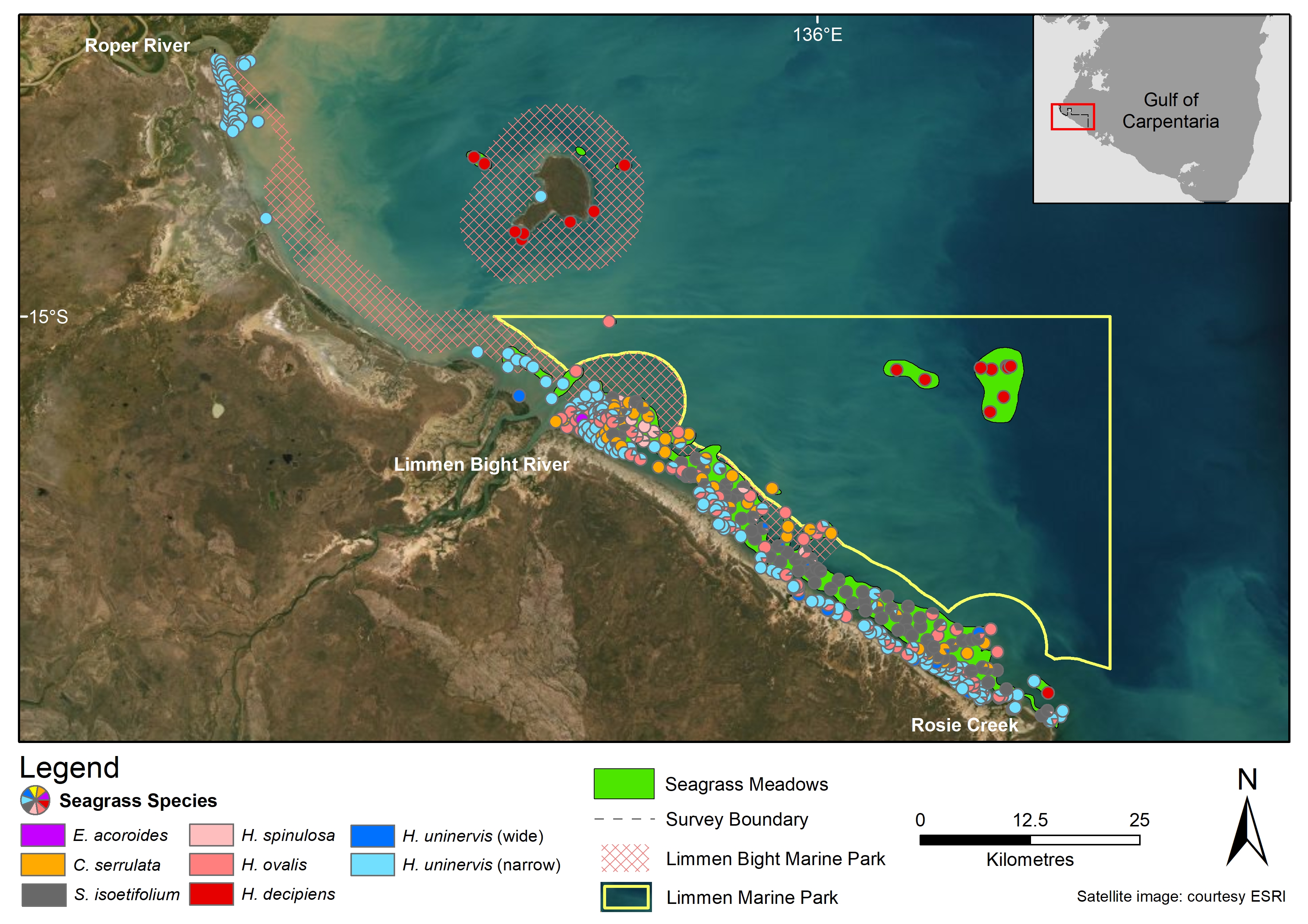
This dataset summarises benthic surveys in Marra Sea Country, including the Limmen Marine Park (Commonwealth) and Limmen Bight Marine Park (Northern Territory) into 4 GIS shapefiles. (1) A point (site) shapefile describes (a) seagrass presence/absence, (b) seagrass species composition, (c) algae cover and (d) benthic macro-invertebrate cover at n=2018 sites surveyed by small vessel and helicopter. (2) A point (site) shapefile describes deep-water (a) seagrass presence/absence, (b) seagrass species composition, (c) algae cover and (d) benthic macro-invertebrate cover at 54 sites surveyed by benthic towed camera and sled net. (3) The meadow shapefile describes attributes of 69 seagrass meadows. (4) The interpolation shapefile describes variation in seagrass biomass across the seagrass meadows. The full report is: Collier C.J., Carter A., Shepherd L., van de Wetering C., Coles R., Evans S., Barrett D., Willan R.C., Groom R. (2022) Benthic habitats of Marra Sea Country - Gulf of Carpentaria. Centre for Tropical Water & Aquatic Marra land and sea country includes coastal waters in the southern Gulf of Carpentaria in the Northern Territory (NT). The Limmen Marine Park (Commonwealth Government) and the Limmen Bight Marine Park (NT Government) are in Marra country. The co-management aspirations identified within the two Marine Park Plans of Management and the Marra Healthy Country Plan include a need to improve information on habitats and key species because they have not been previously mapped. Methods: The sampling methods used to study, describe and monitor seagrass meadows were developed by the TropWATER Seagrass Group and tailored to the location and habitat surveyed; these are described in detail in the relevant publications (https://research.jcu.edu.au/tropwater). Geographic Information System (GIS) All survey data were entered into a Geographic Information System (GIS) developed for Torres Strait using ArcGIS 10.8. Rectified colour satellite imagery of Limmen Bight (Source: Allen Coral Atlas and ESRI), field notes and aerial photographs taken from the helicopter during surveys were used to identify geographical features, such as reef tops, channels and deep-water drop-offs, to assist in determining seagrass meadow boundaries. Four GIS layers were created to describe spatial features of the region: a site layer, seagrass meadow layer, and seagrass biomass interpolation layer. Seagrass site layers Two layers were produced because of additional columns/details on benthic invertebrates that are included in the deep-water shapefile. These layers contains information on data collected at assessment sites and includes: 1. Temporal survey details – Survey date; 2. Spatial position - Latitude/longitude; 3. Survey location; 4. Seagrass information including presence/absence of seagrass, above-ground biomass (total and for each species), percent cover of seagrass at each site and whether individual species were present/absent at a site; 5. Benthic macro-invertebrate information including the percent cover of hard coral, soft coral, sponges and other benthic macro invertebrates (e.g. ascidian, clam) at a site; 6. Algae information including percent cover of algae at a site and percent contribution of algae functional groups to algae cover at a site; 7. Open substrate – the percent cover of the site that had no flora or habitat forming benthic invertebrates present; 8. Dominant sediment type - Sediment type based on grain size visual assessment or deck descriptions. 9. Survey method and vessel 10. Relevant comments and presence/absence of megafauna and animals of interest (sea cucumber, dugong, turtle, dolphin, evidence of dugong feeding trails); 11. Data custodians. Seagrass meadow layer Seagrass presence/absence site data, mapping sites, field notes, and satellite imagery were used to construct meadow boundaries in ArcGIS®. The meadow (polygon) layer provides summary information for all sites within each seagrass meadow, including: 1. Temporal survey details – Survey month and year as individual columns and the survey date (the date range the survey took place); 2. Spatial survey details – Survey location, meadow identification number that identifies the reef name and the meadow number. This allows individual meadows to be compared among years; 3. Survey method; 4. Meadow depth for subtidal meadows. Intertidal: meadow was mapped on an exposed bank during low tide; 5. Species presence – a list of the seagrass species in the meadow; 6. Meadow density – Seagrass meadows were classified as light, moderate, dense based on the mean biomass of the dominant species within the meadow (see Table 3 in Reason et al. 2022). For example, a Thalassia hemprichii dominated meadow would be classed as “light” if the mean meadow biomass was <5 grams dry weight m-2 (g DW m-2), and “dense” if mean meadow biomass was >25 g DW m-2 . 7. Meadow community type – Seagrass meadows were classified into community types according to seagrass species composition within each meadow. Species composition was based on the percent each species’ biomass contributed to mean meadow biomass. A standard nomenclature system was used to categorize each meadow (see Collier et al 2022). 8. Mean meadow biomass measured in g DW m-2 (+ standard error if available); 9. Meadow area (hectares; ha) (+ mapping precision) of each meadow was calculated in the GDA 1994 Geoscience Australia MGA Zone 54 projection using the ‘calculate geometry’ function in ArcMap. Mapping precision estimates (R; in ha) were based on the mapping method used for that meadow (see Collier et al. 2022). Mapping precision estimate was used to calculate an error buffer around each meadow; the area of this buffer is expressed as a meadow reliability estimate (R) in hectares; 10. Any relevant comments; 11. Data custodians. Seagrass biomass interpolation layer An inverse distance weighted (IDW) interpolation was applied to seagrass site data to describe spatial variation in seagrass biomass within seagrass meadows. The interpolation was conducted in ArcMap 10.8. Base map The base map used is courtesy ESRI 2022. Format of the data: This dataset consists of a 2 point layer packages, 1 polygon layer package and 1 raster file with a geographic coordinate system of GDA2020: 1. Marra Sea Country sites 2021.lpk Symbology representing seagrass presence/absence at each survey site 2. Marra Sea Country deepwater sites 2021.lpk Symbology representing seagrass presence/absence at each survey site 3. Marra Sea Country seagrass meadows 2021.lpk 4. Marra Sea Country seagrass biomass interpolation 2021.lpk Symbology representing the spatial variation in seagrass biomass within each seagrass meadow Data dictionary: 1. Marra Sea Country sites 2021 (point data) SITE (numeric) - Unique identifier representing a single sample site MEADOW (text) - Unique identifier representing what meadow the sample site is located in. Blank if sample site is not located within a meadow DATE (numeric) – survey date (day/month/year) MONTH (numeric) – survey month YEAR (numeric) – survey year SURVEY NAME (text) – Name of survey location LOCATION (text) – Name of survey location LATITUDE (numeric) – Site location in decimal degrees south LONGITUDE (numeric) – Site location in decimal degrees east TIME (numeric) – sample time (24 hours; GMT +9:30) (NT time - subtidal sites only) DEPTH (numeric) – depth recorded from vessel depth sounder (metres) for subtidal sites. Intertidal sites depth recorded as 0. DBMSL (numeric) – depth below mean sea level (metres) for subtidal sites. Intertidal sites depth recorded as 0. SUBSTRATE (text) – tags identifying the types of substrates at the sample site. Possible tags are Mud, Sand, Coarse Sand, Silt, Shell, Rock, Reef, Rubble and various combinations. Listed in order from most dominant substrate to least dominant. SEAGRASS_P (numeric) – Absence (0) or Presence (1) of seagrass SEAGRASS_C (numeric) - Estimated % of seagrass cover at sample site SEAGRASS_B (numeric) - Estimated total biomass per square metre for sample site calculated from the mean of three replicate quadrats. Unit is gdw m-2. SEAGRASS_SE (numeric) – standard error of biomass at sample site calculated from the three replicate quadrats used to estimate biomass at a sample site. Unit is gdw m-2. EXCLUDE_FR (numeric) – Include (0) or Exclude (1). Any site identified that needs to be excluded from contributing to the calculation of mean meadow biomass, e.g. where a visual estimate of biomass could not be optioned (i.e. no visibility at the site, only a van Veen sediment grab was used at the site) CR - C. rotundata (numeric). Estimated biomass of Cymodocea rotundata at the sample site. Unit is gdw m-2. CS - C. serrulata (numeric). Estimated biomass of Cymodocea serrulata at the sample site. Unit is gdw m-2. EA - E. acoroides (numeric). Estimated biomass of Enhalus acoroides at the sample site. Unit is gdw m-2. HUT - H. uninervis (narrow) biomass (numeric). Estimated biomass of Halodule uninervis (narrow leaf morphology) at the sample site. Unit is gdw m-2. HUW - H. uninervis (wide) (numeric). Estimated biomass of Halodule uninervis (wide leaf morphology) at the sample site. Unit is gdw m-2. HD - H. decipiens (numeric). Estimated biomass of Halophila decipiens at the sample site. Unit is gdw m-2. HO - H. ovalis (numeric). Estimated biomass of Halophila ovalis at the sample site. Unit is gdw m-2. HS - H. spinulosa (numeric). Estimated biomass of Halophila spinulosa at the sample site. Unit is gdw m-2. HTricost_B - H. tricostata (numeric). Estimated biomass of Halophila tricostata at the sample site. Unit is gdw m-2. SI - S. isoetifolium (numeric). Estimated biomass of Syringodium isoetifolium at the sample site. Unit is gdw m-2. TCilatu_B - T. ciliatum biomass (numeric). Estimated biomass of Thalassodendron ciliatum at the sample site. Unit is gdw m-2. THempric_B - T. hemprichii (numeric). Estimated biomass of Thalassia hemprichii at the sample site. Unit is gdw m-2. ZMueller_B - Z. muelleri biomass (numeric). Estimated biomass of Zostera muelleri at the sample site. Unit is gdw m-2. ALGAE_COVER (numeric) - Estimated % of algae cover at sample site (all algae types grouped) TURF_MAT_A (numeric) – (Turf mat algae % contribution to algae cover). Algae that forms a dense mat on the substrate ERECT_MACROPHYTE (numeric) – (Erect macrophyte algae % contribution to algae cover). Macrophytic algae with an erect growth form and high level of cellular differentiation, e.g. Sargassum, Caulerpa and Galaxaura species ENCRUSTING (numeric) – (Encrusting algae % contribution to algae cover). Algae that grows in sheet-like form attached to the substrate or benthos, e.g. coralline algae. ERECT_CALCAREOUS (numeric) – (Erect calcareous algae % contribution to algae cover). Algae with erect growth form and high level of cellular differentiation containing calcified segments, e.g. Halimeda species. FILAMENTOUS (numeric) – (Filamentous algae % contribution to algae cover). Thin, thread-like algae with little cellular differentiation. *Note: TURF_MAT + ERECT_MACROPHYTE + ENCRUSTING + ERECT_CALCAREOUS + FILAMENTOUS = 100% of algae cover HARD_CORAL (numeric) – (Hard coral %). All scleractinian corals including massive, branching, tabular, digitate and mushroom SOFT_CORAL (numeric) – (Soft coral %). All alcyonarian corals, i.e. corals lacking a hard limestone skeleton SPONGE (numeric) – (Sponge %) OTHER_BMI (numeric) – Any other benthic macro-invertebrates identified, e.g. oysters, ascidians, clams. Other benthic macro-invertebrates are listed in the “comments” attribute for intertidal and shallow subtidal camera drops, and listed as percent cover in the deepwater GIS. OPEN_SUBSTRATE (numeric) – Open substrate, no seagrass, algae or benthic macro-invertebrates at site DUGONG (numeric) - Absence (0) or Presence (1) of dugong/s at site TURTLE (numeric) - Absence (0) or Presence (1) of turtle/s at site DOLPHIN (numeric) - Absence (0) or Presence (1) of dolphin/s at site SEA CUCUMBER (numeric) - Absence (0) or Count (>1) of sea cucumbers at site DFT PRESENT (numeric) - Absence (0) or Presence (1) of dugong feeding trails at site. Only clearly visible and therefore assessed at intertidal sites. Subtidal sites not assessed for DFTs coded as -999 METHOD (text) – e.g. helicopter, walking, hovercraft, boat-based including camera, free diving, scuba diving, van Veen grab, sled net VESSEL (text) – Vessel name (if known) COMMENTS (text) – Any comments for that site AUTHOR (text) – Creator of GIS from the data set CUSTODIAN (text) – Custodian/owner of the data set *Note: SEAGRASS_C + ALGAE_COVER + HARD_CORAL + SOFT_CORAL + SPONGE + OTHER_BMI + OPEN_SUBSTRATE = 100% of benthic cover 2. Marra Sea Country deepwater survey sites 2021 (point data) In addition to the above columns, the additional columns are included in the deepwater site data: CORAL BLEACHING (numeric) - Absence (0), Presence (1) of coral bleaching at site. Sites without coral coded as -999 pc_Anemone (numeric) – Anemone % benthic cover. Soft coral category. pc_Ascidian (numeric) – Ascidian % benthic cover. Other BMI category. pc_Bryozoan (numeric) – Bryozoan % benthic cover. Other BMI category. pc_Crinoids (numeric) – Crinoid % benthic cover. Other BMI category. pc_Gorgonian (numeric) – Gorgonian % benthic cover. Soft coral category. pc_Hydroid (numeric) – Hydroid % benthic cover. Other BMI category. pc_SeaWhip (numeric) – Sea whip % benthic cover. Soft coral category. pc_SCOther (numeric) – Other soft corals % benthic cover. Soft coral category. *Note: pc_Anemone + pc_Gorgonia + pc_SeaWhip + pc_SCOther = SOFT_CORAL % cover *Note: pc_ Ascidian + pc_ Bryozoan + pc_ Crinoids + pc_ Hydroid = OTHER_BMI % cover 3. Marra Sea Country seagrass meadows 2021 (polygon data) ID (numeric) - Unique identifier representing a single meadow SURVEY_NAME (text) – Name of survey location LOCATION (text) – Name of survey location SURVEY_DATE (numeric) – Sample date (day/month/year) MONTH (numeric) – Sample month YEAR (numeric) – Sample year MEADOW_DEPTH (text) – Classified into three categories (intertidal, subtidal, intertidal-subtidal) PERSISTENCE (text) – Meadow form on three categories: enduring, transitory, unknown DENSITY (text) – Meadow density categories (light, moderate, dense) TYPE (text) - Meadow community type determined according to seagrass species composition within the meadow SPECIES (text) – (Seagrass species): seagrass species found within the meadow. Species are recorded as abbreviated species names such as “E. acoroides” TOT_SITES (numeric) – (Number of survey sites): the number of sample sites within the meadow BIOMASS (numeric) – (Seagrass biomass (gdw m-2)): Mean biomass calculated from all sites (BIO_SITES) within an individual meadow SE (numeric) – (Standard Error (gdw m-2)): The error is a calculation of standard error of biomass from all (BIO_SITES) sites within an individual meadow AREA_HA (numeric) – (Meadow area (Ha)): Estimated meadow size (unit: hectares) R_M (numeric) – (Meadow mapping precision (m)): Estimated mapping precision based on mapping method. R_HA (numeric) - (Meadow reliability estimate (Ha)): Meadow reliability estimate (unit: hectares). Expressing the error buffer around each meadow as calculated from the mapping precision estimate SURVEY METHOD (text) – e.g. helicopter, walking, hovercraft, boat-based including camera, free diving, scuba diving, van Veen grab, sled net VESSEL (text) – Vessel name (if known) COMMENTS (text) – Any relevant comments for that meadow UPDATED (date) – The date the shapefile was last updated CUSTODIAN (text) – Custodian/owner of the data set 4. Marra Sea Country biomass interpolation 2021 (interpolation layer) Inverse Distance Weighted interpolation. Band 1: Interpolated biomass in gdw m-2 eAtlas processing: The original data were provided as layer packages which were converted into Shapefiles and Tiff. Minor modifications to the underlying atrribute table on the meadows layer was performed to align the exported shapefile to the data dictionary order. The projection was changed on both the Meadows and Biomass Interpolation layers to allow visualisation on the eAtlas. Location of the data: This dataset is filed in the eAtlas enduring data repository at: data\\custodian\2020-2029-other\GoC_JCU_Murra-Sea-Country-Seagrass_2021

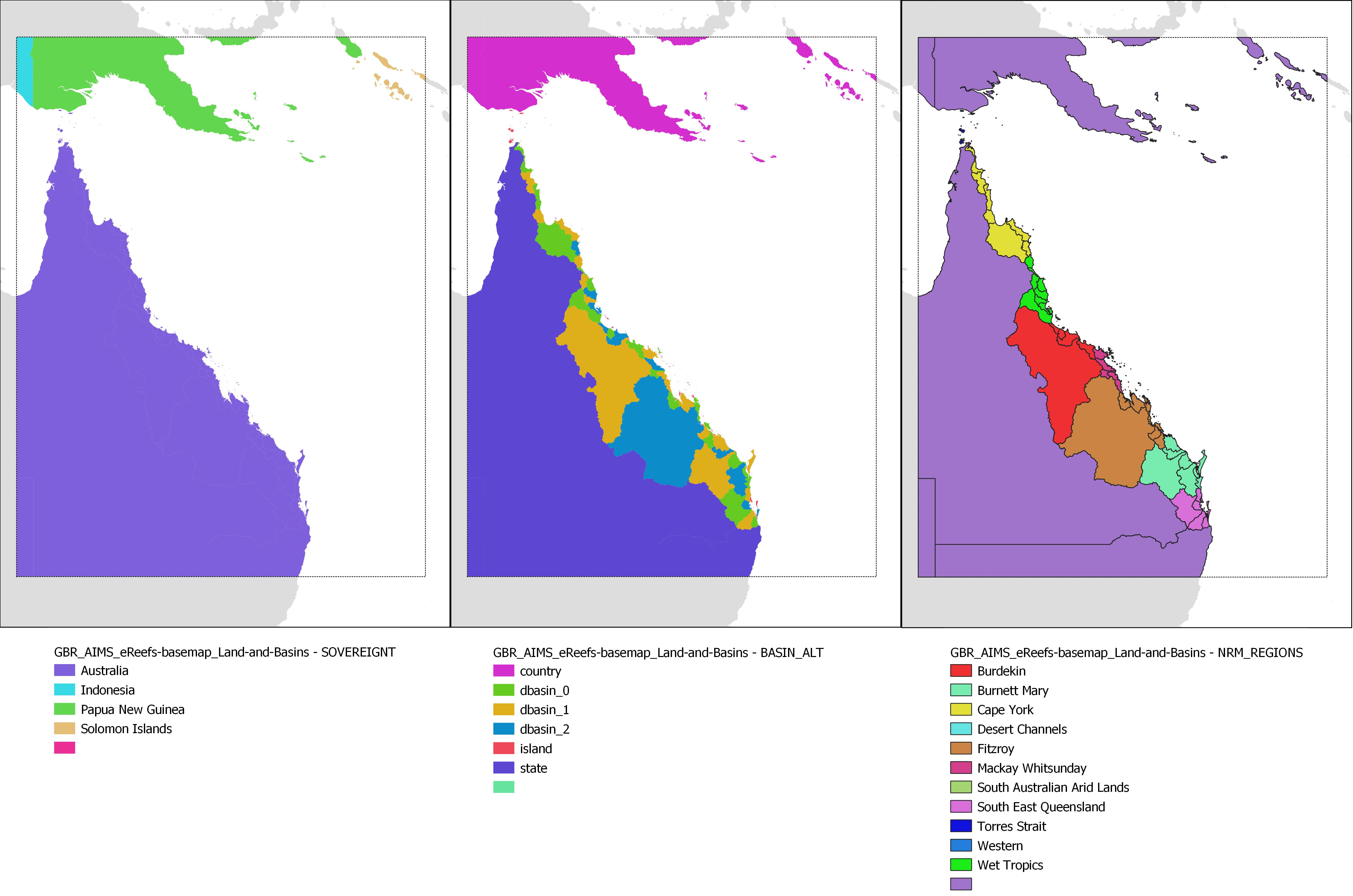
This dataset collection contains GIS layers for creating the AIMS eReefs visualisation maps (https://ereefs.aims.gov.au/). These datasets are useful for creating A4 printed maps of the Great Barrier Reef and the Coral Sea. It contains the following datasets: - Countries - Australia plus surrounding countries at 1:10M scale. Crop of Natural Earth Data 1:10 Admin 0 - Countries dataset. Allows filtering out of surrounding countries. - Cities - 21 Cities along the Queensland coastline. - Basins - Drainage basins adjacent to the Great Barrier Reef along the eastern Queensland coastline. Derived from Geoscience Australia River Basins 1997 dataset. It is a subset and reprojection. - Land and Basins - This layer contains both Queensland and PNG land areas, along with the river basins along the eastern Queensland coastline. This is an integrated layer that represents both the background land area and the river basins all in one layer. This layer saves having to map the land area, then overlay the river basins. In this way each polygon only needs to be rendered once. The goal of this layer is to optmise the rendering time of the eReefs base map. This dataset is made up from the Geoscience Australia Australia's River Basins 1997 dataset for the Queensland coastline and the eastern Queensland basins. PNG is copied from Natural Earth Data 10 m countries dataset. - Rivers - Rivers that drain along the Queensland eastern coast. This is a subset of the Geoscience Australia Geodata Topo 1:5M 2004. - Reefs - Boundaries of reefs in GBR, Torres Strait and Coral Sea. In the Coral Sea it contains the atoll platform boundaries rather than the individual reefs. This is derived from the GBRMPA GBR features dataset, AIMS Torres Strait features dataset and the AIMS Coral Sea features dataset. These were combined and simplified to a scale of 1:1M. Note that this simplification resulted in multiple neighbouring reefs being grouped together. This dataset is intended for visual rendering of maps. - Clip regions - Polygons for clipping eReefs data to the GBR. Also contains approximate polygons for Coral Sea, Torres Strait, PNG and New Caledonia. This was created principally for setting the region attribute for the Reefs dataset, but was made available as it is useful for clipping eReefs data to the GBR for plotting purposes. Methods: Most of the base map layers are derived from a variety of data sources. The full workflow used to transform these source datasets is documented on GitHub (https://github.com/eatlas/GBR_AIMS_eReefs-basemap). Limitations of the data: The datasets in this collection have been cropped and simplified for the purposes of creating low detail printed maps of the GBR. They are not intended for creating a high resolution base map. Format of the data: Shapefile and GeoJSON files. The Cities dataset is provided as a CSV file. Location of the data: This dataset is filed in the eAtlas enduring data repository at: data\custodian\2018-2024-eReefs\GBR_AIMS_eReefs-basemap