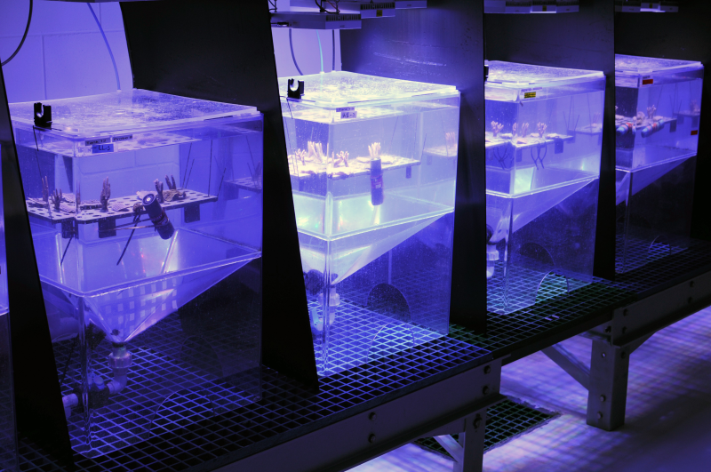
The dataset consists of four data files from a 20-day experiment to investigate different photophysiological responses of two species of coral (Acropora millepora and Pachyseris speciosa) to constant and variable daily light integrals. Methods: Eight partial colonies each of Pachyseris speciosa (from 5 – 8 m depth) and Acropora millepora (from 3 – 5 m depth) were collected from Davies Reef, central Great Barrier Reef, Australia (-18.823390, 147.6518563) in July 2016, and taken to the National Sea Simulator at the Australian Institute of Marine Science (AIMS), Townsville. Experiment consisted of four types of light exposure treatments, wherein nubbins from the partial colonies were either exposed to 20 days of high light (32 mol photons m-2 d-1), low light (6 mol photons m-2 d-1), or alternating variable light treatments. Four sets of photoacclimation and physiological responses were measured and the corresponding data has been placed in four separate csv files; (1) Fluorescence measurements were conducted using a diving pulse-amplitude modulated fluorometer (DPAM). Measurements were taken twice with the DPAM: once at 0.5 h before sunrise, to assess the maximum quantum yield of photosystem II (Fv/Fm), and at noon, after 0.5 h exposure to maximum irradiance, to assess effective quantum yield (PSII). For each nubbin, at least five measurements were taken from different regions on each nubbin and the values averaged. The excitation pressures on PSII, (see Ralph et al. 2016) was assessed to estimate the degree of photoinhibition versus light limitation. Non-photochemical quenching (NPQ), also derived from PAM pre-dawn and noontime measurements based on equations by Genty et al 1987, was measured to assess the amount of excess photon energy dissipated safely as heat. (2) At the end of the experiment, the concentration of chlorophyll a (photosynthetic) and total carotenoids (photosynthetic and photoprotective) of nubbins were compared between treatments. Tissue was removed from the skeleton with an air gun and filtered seawater, and homogenized. The slurry was centrifuged for 6-8 min at 1,500 g and the coral host supernatant was separated from the symbiont pellet. The pellet was then rinsed with filtered seawater and re-centrifuged at 10,000 g for 3 min prior to extraction. Pigments were obtained via a double extraction procedure (1 mL 95% ethanol at 4oC for 20 minutes each, with sonicator), and the absorbance was spectrophotomerically measured at 665, 664, 649 and 470 nm wavelengths. Concentrations of chlorophyll a and total carotenoids (µg/mL) were calculated based on equations by Lichtenthaler (1987) and Ritchie (2008) and standardized to nubbin surface area, which was estimated via a single wax dip protocol (Veal et al 2010). (3) At the end of the experiment, 18 nubbins were selected for respirometry measurements. Their ceramic plugs were carefully cleaned to remove algal growth. Nubbins were individually placed in 634 mL sealed stirred chambers that contained oxygen sensor spots (optodes), and the Firesting hardware/software (Pyroscience, Germany) was used to measure oxygen concentrations within the chambers every minute. Incubations ran for an hour each at ten light levels (0, 15, 40, 80, 120, 200, 300, 500, 700 and 1000 µmol photons m-2 s-1), measured with an upwards facing, calibrated, cosine corrected light sensor (meter LI-250A, sensor LI-192, Li-COR, USA). Water was flushed in the chambers at the beginning of each light level measurement. Rates of oxygen consumption (estimated respiration in the dark) and production (estimated net photosynthesis in the light) were standardized to coral surface area estimates derived from the wax dipping procedure. Photosynthesis to irradiance (P-I) curves were fitted to the data using a hyperbolic tangent fit, as described by Jassby and Platt (1976) using the ‘stats’ package (version 3.6.0) in the statistical platform R (version 3.4.0, R Development Core Team 2017). Parameters for maximum photosynthetic production (Pmax), saturation irradiance (Ik) and dark respiration (Rdark) for each treatment were estimated from fitted models. Net daily oxygen production (Pn) was calculated by predicting production using the P-I curves at actual logged experimental light levels, over a 24 h period. (4) Growth rates of A. millepora were assessed as differences in buoyant weight over time (Davies 1989). Nubbins were individually weighed to the nearest 0.001 g by suspending them on a tray below a semi-micro balance (Shimadzu AUW220D, Japan) in a water bath at ~25 OC. The percent change in buoyant weight between days 8 and 20 was assessed. Literature Cited Lichtenthaler HK. [34] Chlorophylls and carotenoids: Pigments of photosynthetic biomembranes. Methods in Enzymology. 148: Academic Press; 1987. p. 350-82. Ritchie RJ. Universal chlorophyll equations for estimating chlorophylls a, b, c, and d and total chlorophylls in natural assemblages of photosynthetic organisms using acetone, methanol, or ethanol solvents. Photosynthetica. 2008;46(1):115–26. Veal CJ, Holmes G, Nunez M, Hoegh-Guldberg O, Osborn J. A comparative study of methods for surface area and three-dimensional shape measurement of coral skeletons. Limnology and Oceanography: Methods. 2010;8(5):241-53. doi: 10.4319/lom.2010.8.241. Jassby AD, Platt T. Mathematical formulation of the relationship between photosynthesis and light for phytoplankton. Limnology and Oceanography. 1976;21(4):540-7. doi: 10.4319/lo.1976.21.4.0540. Davies S. Short-term growth measurements of corals using an accurate buoyant weighing technique. Marine Biology. 1989;101(3):389–95. doi: 10.1007/BF00428135. Ralph PJ, Hill R, Doblin MA, Davy SK (2016) Theory and application of pulse amplitude modulated chlorophyll fluorometry in coral health assessment. In: Diseases of Coral, pp. 506–523. Format: The dataset consists of four separate components, stored as .csv files, pertaining to the different physiological aspects used to understand coral responses to variable light conditions; fluorometry (85KB), pigment analysis (6KB), respirometry (9KB) and growth (1KB). Data Dictionary: pam.csv - Date: Date of sampling (DD/MM/YY) - Group: Which sampling group the individual was placed in. - Treatment: Which treatment the individual was in, where HL is High Light, LL is Low Light, VLH is Variable Light starting High and VLL is Variable Light starting Low. - Tank: Tank number each nubbin resided in - Species: Either Acropora millepora or Pachyseris speciosa - Coral_ID: Colony identification - Fo_mean: minimum fluorescence yield in dark - Fm_mean: maximum fluorescence yield in dark - DA_yield; Refers to the maximum quantum yield, quantifies the maximum potential for photosynethesis through proportion of available photosystems in a dark-adapted state (dimensionless) - F_mean; steady-state fluorescence yield in light - Fm._mean; maximum fluorescence yield in light - LA_yield: refers to the effective quantum yield, quantifying the relative number of open to closed photosystems in a light-adapted state (dimensionless) - Qm; Excitation pressure of photosystem II, which is a relationship between effective and maximum quantum yields and gives an idea of the relative light-limitation or photoinhibitory stress on the coral (dimensionless) pigments.csv - Treatment: Which treatment the individual was in, where HL is High Light, LL is Low Light, VLH is Variable Light starting High and VLL is Variable Light starting Low. - Tank: Tank number - Species: Either Acropora millepora or Pachyseris speciosa - Coral_ID: Colony identification - Individual_ID: Individual identification - Surface: Relevant for P. speciosa only, refers to whether tissue was taken from the top or the bottom of the nubbin - surfaceArea: Surface area in cm2 - ChlA: estimated total of chlorophyll a (micrograms) per individual coral nubbin - Caro: estimated total of total carotenoids (micrograms) per individual coral nubbin - chlaSA: estimate of chlorophyll a by surface area (micrograms per cm2) per individual coral nubbin - caroSA: estimate of total carotenoids by surface area (micrograms per cm2) per individual coral nubbin - Ratio: Ratio of chlorophyll a to carotenoids respirometry.csv - Date: Date of sampling (DD/MM/YY) - Group: Which sampling group the individual was placed in, based solely on order of respirometry run - Pattern: Whether the treatment was constant (HL or LL) or variable (VLH or VLL) - Treatment: Which treatment the individual was in, where HL is High Light, LL is Low Light, VLH is Variable Light starting High and VLL is Variable Light starting Low - Light: Whether light levels were low or high - Irradiance (umolEm-2s-1); Instantaneous irradiance measurement in micromoles photons per m2 per second - Species: Either Acropora millepora or Pachyseris speciosa - ID: Individual ID - Production_mgO2hr-1: Oxygen production based on respirometry in milligrams of oxygen produced per hour weight.csv (only Acropora millepora in this dataset) - Treatment: Which treatment the individual was in, where HL is High Light, LL is Low Light, VLH is Variable Light starting High and VLL is Variable Light starting Low - Tank: Tank number - Coral_ID: Colony and individual ID - Percent_change: percent change in buoyant weight Data Location: This dataset is filed in the eAtlas enduring data repository at: data\2016-18-NESP-TWQ-2\2.3.1_Benthic-light\AU_NESP-TWQ-2.3.1_AIMS_BenthicLight_experiment2

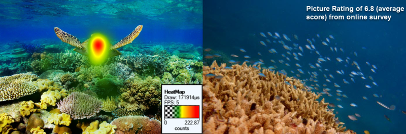
This dataset resulted from two inter-linked research streams. The first stream was related to the application of eye-tracking technology and an online survey in studying natural beauty. The second stream is related to the development of an Artificial Intelligence (AI)-based system recognising and assessing the beauty of natural scenes. Due to differences in data collection and data analysis, details of research methods used for each research stream are described in three separated data records. This record that describes the common elements and goals of the three parts to the research. Within these research streams, three datasets were developed. These include: Eye tracking - containing the outcome documents of eye-tracking experiment conducted within the project framework Online survey - includes a survey format document and three subfolders showing how each section of the survey was designed and outcome of each section (i.e. conjoint analysis, picture rating and open question) Algorithm data reflecting how a computer-based system for automated assessment of image attractiveness is developed Format and methods: The project dataset has multiple parts containing data of different formats and methods. Details of each dataset are discussed in the corresponding data records. Data Dictionary: See data dictionaries in the following data report forms: Becken, S., Connolly R., Stantic B., Scott N., Mandal R., Le D., (2018), Eye-tracking data report form, Griffith Institute for Tourism Research Report No 15. Becken, S., Connolly R., Stantic B., Scott N., Mandal R., Le D., (2018), Online survey data report form, Griffith Institute for Tourism Research Report No 15. Becken, S., Connolly R., Stantic B., Scott N., Mandal R., Le D., (2018), Algorithm data report form, Griffith Institute for Tourism Research Report No 15. References: Further information can be found in the following publication: Becken, S., Connolly R., Stantic B., Scott N., Mandal R., Le D., (2018), Monitoring aesthetic value of the Great Barrier Reef by using innovative technologies and artificial intelligence, Griffith Institute for Tourism Research Report No 15. Becken, S., Connolly R., Stantic B., Scott N., Mandal R., Le D., (2018), Eye-tracking data report form, Griffith Institute for Tourism Research Report No 15. Becken, S., Connolly R., Stantic B., Scott N., Mandal R., Le D., (2018), Online survey data report form, Griffith Institute for Tourism Research Report No 15. Becken, S., Connolly R., Stantic B., Scott N., Mandal R., Le D., (2018), Algorithm data report form, Griffith Institute for Tourism Research Report No 15. Data Location: This dataset is filed in the eAtlas enduring data repository at: data\nesp3\3.2.3_Aesthetic-Values-GBR

This dataset consists of three data files (spreadsheets) from a two month aquarium experiment manipulating pCO2 and light, and measuring the physiological response (photosynthesis, growth, protein and pigment content) of the adult and juvenile stages of two species of tropical corals (Acropora tenuis and A. hyacinthus). Methods: We conducted a two-month, 24-tank experiment at AIMS’s SeaSim facility, in which recently settled juvenile- and adult-colonies of the corals Acropora tenuis and A. hyacinthus were exposed to four light treatments (high, medium, low and variable intensities), fully crossed with two levels of dissolved CO2 (400 and 900 ppm). The four light treatments used in the experiment (low, medium, high and variable) each had 12 hrs of light and a five hour ramp, but at different intensities. The high light treatment had a noon max of 500 µmol photon m-2 s-1 and a DLI of 12.6 mol photon m-2, the medium treatment had a noon max of 300 µmol photon m-2 s-1 and a DLI of 7.56 mol photon m-2, while the low light treatment had a noon max of 100 µmol photon m-2 s-1 and a DLI of 2.52 mol photon m-2. The variable treatment oscillated on a five day cycle, with four days at the low treatment intensity, a ramp day at the medium, then four days at the high treatment intensity. The mean DLI of the variable treatment was therefore the same as medium treatment. Light intensities were checked in each individual aquaria with a calibrated underwater light sensor (Licor, USA). The variable light treatment allowed us to investigate how these corals acclimate to a changing light environment, and to see if responses are due to limitation under low light, or inhibition under high light (i.e. coral responses in the variable treatment would resemble the low or high light treatments), or whether light has a cumulative effect regardless of variability (i.e. coral responses in the variable treatment would resemble the medium light treatment). Adult corals were collected from Davies Reef (18.30 S, 147.23 E) while juveniles were spawned from adults at AIMS’s SeaSim facility. After two months of experiment exposure, growth (change in corallite number) and survivorship were assessed in the juvenile corals from photographs, while growth (buoyant weight changes), and protein and pigment content were assessed in the adults after tissue stripping following standard procedures. Briefly, each adult coral nubbin was water-picked in 10 mL of ultra-filtered seawater (0.04 µm) to remove coral tissue. This tissue slurry was then homogenised and centrifuged to separate coral and symbiont components following. Total coral protein content was quantified from the coral tissue supernatant with the DC protein assay kit (Bio-Rad Laboratories, Australia), while Symbiodinium pigments in the pellet were determined spectrophotometrically (Lichtenthaler 1987, Richie 2008). Protein content was standardised to nubbin surface area, estimated with the single wax-dipping technique (Veal et al. 2010), while pigment content was standardised by nubbin surface area, as well as by protein content. A series of photophysiological measurements for the effective (PhiPSII) and maximum (Fv/Fm) quantum yield of photosystem II were made on the adults with a pulse amplitude modulated fluorometer over the final ten days of the experiment. Photosynthetic pressure (Qm: 1 - PhiPSII / Fv/Fm) and relative electron transport rate (rETR: PhiPSII * PAR) were calculated (Ralph et al. 2016) to see how they were responding to their light environment. References: Lichtenthaler HK (1987) Chlorophylls and carotenoids: Pigments of photosynthetic biomembranes. Methods in Enzymology, 148, 350–382. Ralph PJ, Hill R, Doblin MA, Davy SK (2016) Theory and application of pulse amplitude modulated chlorophyll fluorometry in coral health assessment. In: Diseases of Coral, pp. 506–523. Ritchie RJ (2008) Universal chlorophyll equations for estimating chlorophylls a, b, c, and d and total chlorophylls in natural assemblages of photosynthetic organisms using acetone, methanol, or ethanol solvents. Photosynthetica, 46, 115–126. Veal CJ, Carmi M, Fine M, Hoegh-Guldberg O (2010) Increasing the accuracy of surface area estimation using single wax dipping of coral fragments. Coral Reefs, 29, 893–897.

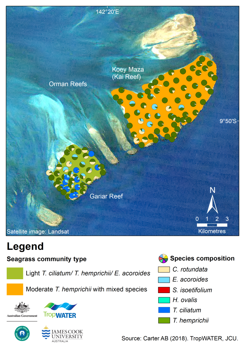
This dataset summarises intertidal benthic surveys of Kai and Gariar Reefs (Orman Reefs, Torres Strait) in November 2018 into 3 GIS shapefiles. (1) The site shapefile describes (a) seagrass presence/absence and (b) species composition at 124 sites. (2) The meadow shapefile describes seagrass communities for the two reef-top meadows. (3) The interpolation shapefile describes variation in seagrass biomass across sites for the two reef-top meadows. This project is part of ongoing long-term monitoring of intertidal reef-top seagrass in Torres Strait, and follows on from a baseline survey of Orman Reefs in September 2017. It describes seagrasses at two of the largest reefs in the Orman Reef complex – Kai (Koey Maza) and Gariar Reefs. This monitoring provides essential information to the TSRA, Australian and Queensland governments for dugong and turtle management plans, complimenting dugong and turtle research studies in the region. Methods: The sampling methods used to study, describe and monitors seagrass meadows were developed by the TropWATER Seagrass Group and tailored to the location and habitat surveyed; these are described in detail in the relevant publications (https://research.jcu.edu.au/tropwater). 1 Location Sites were surveyed by helicopter. At each site latitude and longitude was recorded by GPS. Sediment type was recorded. 2 Seagrass metrics At each site observers estimated the percent cover of seagrass, then for three quadrats within each site, ranked seagrass biomass and estimated the percent contribution of each species to that biomass. Helicopter was used for the intertidal surveys following TropWATER’s methods to assess areas at high risk from shipping accidents in Torres Strait (Carter et al. 2013). At each site the helicopter comes into a low hover and seagrass was ranked and species composition estimated from three 0.25 m2 quadrats placed randomly within a 10m2 circular area. Seagrass above-ground biomass was determined using the “visual estimates of biomass” technique (Mellors 1991) using trained observers. This involves ranking seagrass biomass while referring to a series of quadrat photographs of similar seagrass habitats for which the above-ground biomass has been previously measured. Three separate biomass scales are used: low biomass, high biomass, and Enhalus biomass. The percent contribution of each seagrass species to total above-ground biomass within each quadrat is also recorded. At the completion of sampling each observer ranks a series of calibration quadrats. A linear regression is then calculated for the relationship between the observer ranks and the harvested values. This regression is used to calibrate above-ground biomass estimates for all ranks made by that observer during the survey. Biomass ranks are then converted to above-ground biomass in grams dry weight per square metre (g DW m-2). 3 Benthic macro-invertebrates At each site a visual estimate of benthic macro-invertebrate (BMI) percent cover was recorded each site according to four broad taxonomic groups: • Hard coral – All scleractinian corals including massive, branching, tabular, digitate and mushroom. • Soft coral – All alcyonarian corals, i.e. corals lacking a hard limestone skeleton. • Sponge. • Other BMI – Any other BMI identified, e.g. hydroid, ascidian, barnacle, oyster, mollusc. Other BMI are listed in the “comments” column of the GIS site layer. 4 Algae A visual estimate of algae percent cover was recorded at each site. When present, algae were categorised into five functional groups and the percent contribution of each functional group was estimated: • Erect macrophyte – Macrophytic algae with an erect growth form and high level of cellular differentiation, e.g. Sargassum, Caulerpa and Galaxaura species. • Erect calcareous – Algae with erect growth form and high level of cellular differentiation containing calcified segments, e.g. Halimeda species. • Filamentous – Thin, thread-like algae with little cellular differentiation. • Encrusting – Algae that grows in sheet-like form attached to the substrate or benthos, e.g. coralline algae. • Turf mat – Algae that forms a dense mat on the substrate. All survey data were entered into a Geographic Information System (GIS) developed for Torres Strait using ArcGIS 10.4. Rectified colour satellite imagery of Orman Reefs (Source: ESRI, Landsat 2018), field notes and aerial photographs taken from the helicopter during surveys were used to identify geographical features, such as reef tops, channels and deep-water drop-offs, to assist in determining seagrass meadow boundaries. Three GIS layers were created to describe spatial features of the region: a site layer, seagrass meadow layer, and seagrass biomass interpolation layer. Site layer This layer contains data collected at each site, including: • Temporal details – survey date. • Spatial details – latitude/longitude. • Habitat information – sediment type; seagrass information including presence/absence and above-ground biomass (total and for each species); percent cover of seagrass, algae, hard coral, soft coral, sponges, other BMI, and open substrate; percent contribution of algae functional groups to algae cover. • Sampling method and any relevant comments. Seagrass meadow layer Seagrass presence/absence site data, mapping sites, field notes, and satellite imagery were used to construct meadow boundaries in ArcGIS®. The meadow (polygon) layer provides summary information for all sites within the meadow, including: 1. Habitat information – seagrass species present, meadow community type, meadow cover, mean meadow biomass ± standard error (SE), meadow area ± reliability estimate (R), and number of sites within the meadow. 2. A meadow identification number and reef name; this allows individual meadows to be compared among years. 3. Sampling methods. Meadow community type was determined according to seagrass species composition within each meadow. Species composition was based on the percent each species’ biomass contributed to mean meadow biomass. A standard nomenclature system was used to categorize each meadow (Table 1). This nomenclature also included a measure of meadow density categories (light, moderate, dense) determined by mean biomass and the dominant species within the meadow (Table 2). Mapping precision estimates (R; in metres) were based on the mapping method used for that meadow (Table 3). Mapping precision estimates ranged from 10-50m for intertidal seagrass meadows and up to 100m for meadow mapping precision estimates based on the distance between sites with and without seagrass. Mapping precision estimate was used to calculate an error buffer around each meadow; the area of this buffer is expressed as a meadow reliability estimate (R) in hectares. Meadow area and error buffers were determined in hectares using the calculate geometry function in ArcGIS. Table 1. Nomenclature for seagrass community types. Community type (Species composition) Species A (Species A is 90-100% of composition) Species A with Species B (Species A is 60-90% of composition) Species A with Species B/Species C (Species A is 50% of composition) Species A/Species B (Species A is 40-60% of composition) Table 2. Density categories and mean above-ground biomass ranges for each species used in determining seagrass community density. Species: H. ovalis Categories: Light (<1), Moderate (1 - 5), Dense (>5) Species: C. serrulata, C. rotundata, S. isoetifolium, T. hemprichii Categories: Light (<5), Moderate (5 - 25), Dense (>25) Species: E. acoroides, T. ciliatum Categories: Light (<40), Moderate (40 - 100), Dense (>100) Table 3. Mapping precision and methods for seagrass meadows. Mapping precision: Mapping method 10-20 m: - Meadow boundaries mapped in detail by GPS from helicopter - Intertidal meadows completely exposed or visible at low tide - Relatively high density of mapping and survey sites - Recent aerial photography and satellite imagery aided in mapping 50-100 m: - Meadow boundaries determined from helicopter and camera - Inshore boundaries mapped from helicopter - Offshore boundaries interpreted from survey sites and satellite imagery - Relatively high density of mapping and survey sites Seagrass biomass interpolation layer An inverse distance weighted (IDW) interpolation was applied to seagrass site data to describe spatial variation in seagrass biomass across Kai and Gariar Reef meadows. The interpolation was conducted in ArcMap 10.4. Format: This dataset consists of 3 shapefiles with a spatial reference of GDA94. Meadow shapefile 1. Orman Reefs seagrass community type 2018.lpk Includes 2 individual seagrass meadows at Kai and Gariar Reefs mapped in 2018 with information including individual meadow ID, meadow mean seagrass biomass (g DW m-2) ± SE, number of sites surveyed, seagrass cover, meadow area ± R, seagrass community type, seagrass species present, survey dates, survey method, and data author. ESRI and Landsat satellite image basemaps were used as background source data to check meadow and site boundaries, and re-map where required. 2. Orman Reefs seagrass biomass interpolation 2018.lpk An inverse distance weighted (IDW) interpolation was applied to seagrass site data to describe spatial variation in biomass across each meadow at Kai and Gariar Reefs. Site shapefile Includes information including latitude/longitude, seagrass presence/absence, algae and benthic macro-invertebrate percent cover, percent cover of algae functional groups, individual seagrass species biomass, survey date, survey method, and data author. These shapefiles have been presented as 2 layer packages based on symbology from specific columns: 1. Orman Reefs seagrass present absent intertidal 2018.lpk 2. Orman Reefs seagrass species composition 2018.lpk eAtlas Processing: The original data was provided as ArcMap Layer Packages which were converted to open formats (Shapefile, CSV and GeoTiff) for use in the eAtlas mapping system and as part of the dataset download. These conversion were performed with no modifications to the underlying data. References: An assessment of seagrass condition for Kai and Gariar Reefs, and for all of Torres Strait, can be found in this publication: Carter AB, Mellors JM, Reason C, & Rasheed MA (2019). ‘Torres Strait Seagrass 2019 Report Card’. Centre for Tropical Water & Aquatic Ecosystem Research Publication 19/16, James Cook University, Cairns Data Location: This dataset is filed in the eAtlas enduring data repository at: data/TSRA_2018-22/TS_JCU_Orman-Reefs_2018

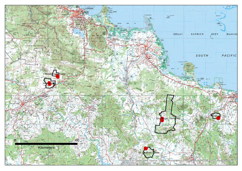
An updated version of this dataset is available at https://eatlas.org.au/data/uuid/38b496a3-3fba-42e7-b904-902f68040c85 Key Gully monitoring localities (headcuts and monitoring instrumentation) and outlines of the properties within which they are located. The data in presented in this metadata are part of a larger collection and are intended to be viewed in the context of the project. For further information on the project, view the parent metadata record: Demonstration and evaluation of gully remediation on downstream water quality and agricultural production in GBR rangelands (NESP TWQ 2.1.4, CSIRO) Methods: Key Gully Localities were extracted from the 2017 or 2018 RTK GPS surveys for each gully site (see Site_Configuration_and_Survey). Property Boundaries were generated by extracting polygons from the 2016 Digital Cadastre Database (DCDB) and simplifying to a single polygon. Area in hectares was calculated and appended to polygon attributes. KMZ’s are exported version of the original ArcGIS shapefiles Format: This data collection consists of two shapefiles (zipped) and two equivalent KMZ files with the following names: NESP_Gully_Key_localities Key gully localities include the RTK GP location of the instrumentation and the RTK GPS location of the nickpoint in the gully headcut rim. NESP_Gully_Property_Boundaries Boundaries for the properties on which the paired control/treatment gullies are located. Data Dictionary: Attributes for Property_Boundaries.shp include property NAME and the area in hectares (AREA_HA). Attributes for Key Locations include X,Y (MGA94 Z55) and Z (AHD) Timestamp associated when RTK surveyed Type- HEADCUT, INSTR Survey – type of survey and year, APPROX is best guess from Lidar or GoogleEarth Site_Code – short form code for sites where MIV = Minnievale MV = Meadowvale MW = Mount Wickham SB = Strathbogie VP = Virginia Park <T/C> - Treatment/Control Property – Full name of property Treat_type – Treatment or control References: Bartley, Rebecca; Hawdon, Aaron; Henderson, Anne; Wilkinson, Scott; Goodwin, Nicholas; Abbott, Brett; Baker, Brett; Matthews, Mel; Boadle, David; Jarihani, Ben (Abdollah). (2018) Quantifying the effectiveness of gully remediation on off-site water quality: preliminary results from demonstration sites in the Burdekin catchment (second wet season). RRRC: NESP and CSIRO. csiro:EP184204. Data Location: This dataset is filed in the eAtlas enduring data repository at: data\NESP2\2.1.4_Gully-remediation-effectiveness

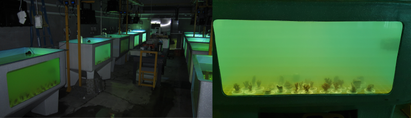
This dataset consists of one data file (spreadsheet) from a 28-d experiment examining sediment-induced changes in the spectral quality and quantity of light on three coral species (Acropora millepora, Pocillopora verrucosa and Montipora aequituberculata) and one encrusting sponge species (Cliona orientalis). The aim of the study was to use ecologically relevant turbidity and light profiles obtained from field-based data to test the effects of sediment induced spectral shifts and quantities of light on corals and sponges. Data from this experiment will help to derive more realistic thresholds to be applied during dredging operations. Methods: Three coral species (Acropora millepora, Pocillopora verrucosa and Montipora aequituberculata) and one encrusting sponge species (Cliona orientalis) were used in SeaSim experiments to examine the effects of sediment induced changes in the quality and quantity of light. A. millepora and M. aequituberculata were collected from Falcon Island (18° 45’ 56.4”S; 146° 32’ 02.7”) and P. verrucosa and C. orientalis were collected from Pelorus Island (18° 45’ 36.7”S; 146° 29’18.5” E). Corals were exposed to 5 different nominal suspended sediment concentrations (nominal SSC of 2.5, 5, 7.5, 10 and 15), with corresponding light profiles, for 28 days. Nephelometers used in the experimental tanks to maintain SSCs were calibrated with Formazin and set to measure Formazin Nephelometric Units (FNU), with water samples taken throughout the experiment (n=12) to relate FNU to SSCs (mg L-1). The gravimetric SSC was determined by filtering water samples (250 mL) through pre-weighed 0.4 µm polycarbonate filters, which were then rinsed with deionized water, dried at 60°C for 24 h and re-weighed. Photosynthetic active radiation (PAR) measurements were taken with a Jaz light meter (Jaz-ULM-200, Ocean Optics, the Netherlands) at peak intensity (12:00), with corresponding daily light integral (DLI) measurements obtained from the ramping profiles extracted from the programable logistic controller (PLC). Several response variables were measured at the end of the 28-d experiment: color (mean grey pixel), symbiont density (total Zoox and Zoox/cm2), chlorophyll a content (µg/cm2 and pg/cell), percent total lipids, ratio of storage to structural lipids (Stor:Struct) and lipid classes (WAX, TAG, FFA, ST, AMPL, PE, PSPI, PC, LPC). All species were photographed using a high-resolution digital camera (Nikon D810) with the following settings: ISO-100, F-29 and shutter speed 1/200. Changes in colour were examined using the hitogram function in ImageJ to obain mean pixel intensity values on a black and white scale (range 0-255) of representative live tissue, as previously described (Bessell-Browne et al., 2017). Surface area (cm2) of the corals were calculated using the wax dipping method (Stimson and Kinzie, 1991). This value was used to standardize zooxanthellae density and chlorophyll concentrations. To determine symbiotic zooxanthellae density, a volume of 0.4 mm3 from each blastate aliquot was counted six times using a Neubauer haemocytometer containing 8 µL of homogenised solution. Pigments were extracted using 95% ethanol and analysed on a Power Wave Microplate Scanning Spectrophotometer (BIO-TEK® Instruments, Inc., Vermont USA) as previously described (Pineda et al., 2016). For lipid analyses, total lipids and lipid classes were acquired by extracting freeze-dried samples following the air-spraying method procedures of (Conlan et al. 2017). Response data for all coral species can be found in the ‘coral’ tab, while the data for C. orientalis can be found in the ‘Cliona’ tab. Format: This dataset contains a single Excel file with a size of 96 KB. Data Dictionary: -SampleID: individual ID given to each replicate of the study -Species: Acropora millepora, Pocillopora verrucosa, Montipora aequituberculata -Tank/Ta: holding, 1 -10 -Nominal SSC: nominal suspended sediment concentration selected in the spectral model -Gravimetric SSC: actual suspended sediment concentration (mg L-1) corals/sponges were exposed to -PAR: maximum light intensity (photosynthetic active radiation; µmol quanta m-2 s-1) corals/sponges were exposed to -DLI: daily light integral (µmol quanta m-2 s-1) corals/sponges were exposed to -Time: day sampled -SA(cm2): surface area of the coral, calculated using the wax dipping method and used to standardize zooxanthellae density and chlorophyll concentrations. -Density of Zoox/cm2: density of zooxanthellae per cm2 tissue -Total Zoox: total number of zooxanthellae -pg Chl a/cell: picograms of chlorophyll a per zooxanthellae cell -Total Chl a: total amount of chlorophyll a per cm2 tissue -Mean grey pixel: mean grey pixel intensity value from imageJ analysis (0=black, 255=white) -%Lipid: the percent total lipid -WAX: percent wax ester (lipid class) -TAG: percent triacylglycerol (lipid class) -FFA: percent free fatty acid (lipid class) -ST: percent sterol (lipid class) -AMPL: percent acetone mobile polar lipid (lipid class) -PE: percent phosphatidylethanolaimine (lipid class) -PSPI: percent phosphatidylserine-phosphatidylinositol (lipid class) -PC: percent phosphatidylcholine (lipid class) -LPC: percent lyso-phosphatidylcholine (lipid class) Stor:Struct: ratio of storage (WAX, TAG, FFA) to structural lipids (all other classes listed) References: Stimson, J., and Kinzie, R.A. (1991). The temporal pattern and rate of release of zooxanthellae from the reef coral Pocillopora damicornis (Linnaeus) under nitrogen-enrichment and control conditions. Journal of Experimental Marine Biology and Ecology 153, 63-74. Bessell-Browne, P., Negri, A.P., Fisher, R., Clode, P.L., Duckworth, A., and Jones, R. (2017a). Impacts of turbidity on corals: The relative importance of light limitation and suspended sediments. Mar Pollut Bull 117, 161-170. Pineda, M.C., Strehlow, B., Duckworth, A., Doyle, J., Jones, R., and Webster, N.S. (2016). Effects of light attenuation on the sponge holobiont- implications for dredging management. Sci Rep 6, 39038. Conlan, J.A., Rocker, M.M., and Francis, D.S. (2017). A comparison of two common sample preparation techniques for lipid and fatty acid analysis in three different coral morphotypes reveals quantitative and qualitative differences. PeerJ 5, e3645. Data Location: This dataset is filed in the eAtlas enduring data repository at: data\nesp2\2.1.9_Dredging-marine-response

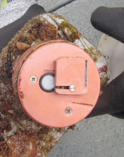
This dataset contains benthic photosynthetically active radiation (PAR; bPAR) at the Q-IMOS Myrmidon, Palm Passage and Heron Island South mooring stations from May 2016 through to November 2017. This dataset was collected to provide in situ reference data for calibration/validation of a remote sensing ocean color model to estimate bPAR (benthic photosynthetically active radiation) as part of NESP Tropical Water Quality Hub project 2.3.1. The mooring is maintained as part of the Queensland IMOS (Q-IMOS) mooring network, which collects oceanographic and water quality data at several stations. bPAR sensors were installed at four stations: Myrmidon (MYD), Palm Passage (PPS), Heron Island South (HIS) and Yongala (YGL). Methods: A WETLabs Environmental Characterization Optics (ECO) PARSB sensor was deployed and clamp-mounted to a permanent mooring wire at a fixed depth within the water column in each of three mooring sites, Myrmidon (MYD), Palm Passage (PPS), and Heron Island South (HIS). Each PAR sensor was programmed to collect 5-second blocks of data every 15 minutes. At the fourth site, Yongala (YGL), a SEABIRD SBE16PLUS V2 SEACAT profiler with PARSB auxiliary sensor “facing” upward was deployed 0.5 m above the bottom substrate. After each period of deployment, data were downloaded and the instrument’s optical component was checked, characterized and tested to ensure the quality and validity of the data between deployments. For each recovery period, the data were analysed and quality controlled such that: (i) data records in the beginning and end of each deployment were excluded to ensure that only stable PAR measurements were included in the analysis, (ii) data points when instrument failure was experienced due to instrument’s internal battery power problems were also excluded. Night-time values were forced to zero by applying an offset based on the dark count readings of the sensor for each deployment period. Summary of mooring stations and in situ data collection Mooring station: YGL Latitude: (°S) -19.302 Longitude: (°E) 147.621 Region: Shallow inshore, seasonally turbid Nominal station Depth: 30m Deployment start:19 Sep 2015 Mooring station: PPS Latitude (°S): -18.308 Longitude (°E): 147.167 Region: Deep, outer shelf, clear oceanic Nominal station Depth: 70m Deployment start: 28 May 2016 Mooring station: MYD Latitude (°S): -18.220 Longitude (°E): 147.344 Region: Deep, shelf edge, clear oceanic Nominal station Depth: 192m Deployment start: 25 May 2016 Mooring station: HIS Latitude (°S): -23.513 Longitude (°E): 151.955 Region: Shallow inshore, intermediate Nominal station Depth: 46m Deployment start: 03 Apr 2016 Data Dictionary: - bPAR: benthic photosynthetically available radiation - bPARoffset: offset (i.e., night time dark readings) corrected bPAR values Data Location: This dataset is filed in the eAtlas enduring data repository at: data\nesp2\2.3.1_Benthic-light

This dataset contains RTK GPS Data collected between April, 2017 and March, 2018 for 5 paired Control/Treatment gully sites being monitored as part of NESP Project 2.1.4 (Demonstration and evaluation of gully remediation on downstream water quality and agricultural production in GBR rangelands). The key question being asked is “is there measurable improvement in the erosion and water quality leaving remediated gully sites compared to sites left untreated?” The monitoring approach uses a modified BACI (Before after control impact) design. The data in presented in this metadata are part of a larger collection and are intended to be viewed in the context of the project. For further information on the project, view the parent metadata record: Demonstration and evaluation of gully remediation on downstream water quality and agricultural production in GBR rangelands (NESP TWQ 2.1.4, CSIRO). Monitoring of these sites is continuing as part of NESP TWQ Project 5.9. Any temporal extensions to this dataset will be linked to from this record. Methods: RTK (Real time kinematic) GPS system (Ashtech, ProMark 200), set with a tolerance of +/- 12mm in the horizontal plane and +/- 15mm in the vertical, was used to survey the monitored gullies. The initial location of the base station was determined using a 10-minute average. All permanent infrastructure such as survey markers, fences, and instrumentation. Gully features such as headcut rims, long sections and cross sections (at key locations such as near instrumentation) were captured. Raw GPS data files were converted to text, imported to Excel for attribute assignments, and then imported to ArcGIS for conversion to shapefile format. Format: This data collection consists of 5 zip files (one for each paired gully monitoring site). Zip files are named according to the property on which they are located. Each zip file contains two shapefiles with detailed RTK GPS survey data from either 2017 or 2018 for the Control and Treatment gullies. Survey point types include Reference markers, gully cross sections, long sections and the gully headcut. Data Dictionary: Attributes for each point include Easting (E) and Northing (N) location info (MGA94 Z55, AHD), descriptive text (Comment), horizontal accuracy (HRMS), vertical accuracy (VRMS), RTK Fix or Float status (STATUS), Number of satellites (SATS), 3D position dilution of precision (PDOP), horizontal dilution of precision (HDOP), Vertical dilution of precision (VDOP), time and date of survey point(Timestamp), and Point type (Type). More information on Dilution of Precision can be found here: https://en.wikipedia.org/wiki/Dilution_of_precision_(navigation) Point Types include REF and BASEREF - Reference markers include permanent survey markers XSREF - Cross Section Transect markers VEGREF - vegetation transect markers STRUCTREF) - Structure markers INSTRREF - location of instrumentation TLSREF - Laser scanner permanent markers gully cross sections (XS) LS - long sections RIM - headcut rim RIMNICK - headcut nickpoint Site_Code used for file names is as follows: MIV = Minnievale MV = Meadowvale MW = Mount Wickham SB = Strathbogie VP = Virginia Park <T/C> - Treatment/Control References: Bartley, Rebecca; Hawdon, Aaron; Henderson, Anne; Wilkinson, Scott; Goodwin, Nicholas; Abbott, Brett; Baker, Brett; Matthews, Mel; Boadle, David; Jarihani, Ben (Abdollah). Quantifying the effectiveness of gully remediation on off-site water quality: preliminary results from demonstration sites in the Burdekin catchment (second wet season). RRRC: NESP and CSIRO; 2018. csiro:EP184204. Data Location: This dataset is filed in the eAtlas enduring data repository at: data\nesp2\2.1.4 Gully-remediation-effectiveness

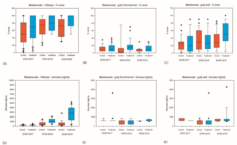
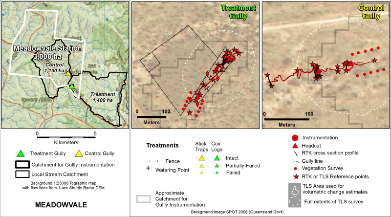
This dataset contains Vegetation and Biomass monitoring data collected for the NESP Project 2.1.4 (Demonstration and evaluation of gully remediation on downstream water quality and agricultural production in GBR rangelands). The aim of the vegetation monitoring in relation to this project is to track change in biomass and species composition over time on hillslope areas above gully erosion within control and treatment sites (treatments vary), linking to changes in downstream water quality. Data is from control and treatment gully sites on commercial grazing properties in the Burdekin being monitored as part of NESP Project 2.1.4. The data in presented in this metadata are part of a larger collection and are intended to be viewed in the context of the project. For further information on the project, view the parent metadata record: Demonstration and evaluation of gully remediation on downstream water quality and agricultural production in GBR rangelands (NESP TWQ 2.1.4, CSIRO) Monitoring of these sites is continuing as part of NESP TWQ Project 5.9. Any temporal extensions to this dataset will be linked to from this record. BOTANAL files describe the biomass, species composition and species attributes such as basal area and cover for hillslope areas above gully erosion sites. PATCHKEY files describe the landscape condition (proportional) of vegetation patches for hillslope areas above gully erosion sites. And BIOMASS files describe the cover and biomass within the gully. Methods: Vegetation metrics were measured on the hillslope above each of the NESP gullies at the end of the dry season (‘EOD’, October–November) and then again at the end of the wet season (‘EOW’, April). Measurements were initiated in November 2016 at all sites except Mt Wickham which started in August 2018. Landscape and vegetation condition transects were installed upslope of the uppermost head section on both the treated and control gullies at all sites (Figure 8). Transects were run along slope contours and varied in length and spacing for each site depending on gully-head catchment size. Four to five transects were used at each treatment and control location. Each transect has a permanent marker at the beginning and end to facilitate repeat measures. Pasture metrics were recorded along each transect using a 1m2 quadrat based on the methods of Tothill et al., (1992), with placement of quadrats dependent on transect length at each site (30 quadrats were sampled for each treatment/control area). Metrics included the main pasture species and/or functional group composition and frequency, above-ground pasture biomass (DMY), total cover, litter cover, basal-area %, defoliation level and key soil surface condition metrics (Tongway and Hindley, 1995). In addition landscape condition was calculated along each transect using PATCHKEY (Abbott and Corfield, 2012). The condition assessments were aggregated to reflect ABCD landscape condition as used across grazed landscapes in the GBR catchments (Aisthorp and Paton, 2004; Chilcott et al., 2005; Bartley et al., 2014). Cover and biomass estimates were calibrated against standard quadrats taken at each site using classified quadrat photographs. Biomass standards were oven dried to attain dry matter yield, removing vegetation water retention error between treatments. A real time kinematic (RTK) survey ran from upslope of the vegetation survey to the valley section for each gully system. Gully vegetation cover and biomass were also measured within each gully, on the gully walls and gully floor. Sampling was initiated at the end of the first wet season (April 2017) for all sites except Mt Wickham which started in August 2018. The sampling methodology was very similar to the hillslope survey. A minimum of three transects were measured across each gully, representative of the head, middle and valley sections. At each transect, % cover, biomass and dominant cover type was assessed using 0.25 m2 (0.5 x 0.5m) quadrats. Three quadrats were assessed on each wall (six in total) and six quadrats assessed in the deepest part of the channel in the gully floor. Box plots of the % cover and biomass data at the end of each wet season for control and treatment sites were analysed using Sigmaplot Version 14. In most cases a t-test for means and non-parametric Mann-Whitney rank sum test were conducted to evaluate differences between treatment and control sites PATCHKEY data was collected at 5 parallel fixed transects above gully locations (hillslope area) – length and spacing of transects varied between sites dependant on hillslope size. PATCHKEY data was collected digitally using custom software on handheld android device. Survey occurs each year before and after wet season. Biomass is calibrated against cut and dried samples and cover is calibrated against classified quadrat photos – per collector. PATCHKEY is used to derive landscape condition from vegetation/grazed patches using vegetation and soil components to derive a condition state – it can be directly aggregated to match ABCD landscape condition. Condition state changes can be measured over time and related to water quality downstream. BOTANAL is a comprehensive sampling and computing procedure for estimating pasture biomass and species composition (Tothill et al 1992) – these files describe the biomass, species composition and species attributes such as basal area and cover for hillslope areas above gully erosion sites. Limitations of the data: This dataset contains Vegetation monitoring data collected at these gully sites for end of the dry season (‘EOD’, October–November) for Hillslope only and then again at the end of the wet season (‘EOW’, April) for Hillslope and Gully over three reporting periods 2016-2017, 2017-2018 and 2018-2019. Measurements were initiated in November (EOD) 2016 at all sites except Mt Wickham which started in August (EOD) 2018. Format: This data collection consists of 3 zip files each monitoring period. Each zip file contains 4 CSV files and one Microsoft Excel file: Two BOTANAL CSV files – 1 EOD and 1 EOW, Two PATCHKEY CSV files – 1 EOD and 1 EOW End of Wet season Gully_veg measurements are stored by season as Microsoft Excel file. Individual tabs for each site record the raw data as captured in the field. The “Stnds” tab calculated the calibration from BIO code to actual biomass. The “all_for_stats” sheet is the intermediate sheet for collation of data in “Wall” and “Channel” sheets ready for analysis in stats package. “Summary” tab contains summary data for the report. Data Dictionary: BOTANAL CSV headers: ID: Unique identifier for sample USER: Collector name/initials SITE: Site name (abbreviation) TRAN: Transect number (numbered from nearest to gully) QUAD: Quadrat number per transect (numbered from left side – looking downhill) DATE: Date and time SP1 to SP5: Species name abbreviated using first two letters of genus and first three of species name eg. Bothriochloa pertusa = boper. Species recorded in order of highest biomass represented. SPP1 to SPP5: Species proportion by weight of quadrat for each of species 1 to 5 YIELD: Total biomass estimate for quadrat in kg/ha DEFOL: Estimated cattle defoliation of the pasture within quadrat. Categorical – 1=0-5%, 2=5-25%, 3=25-50%, 4=50-75% and 5=75-100% BASAL: Estimated basal area of Perennial tussock grasses. % of quad COVER: Foliage projected cover % of quad LITTER: Litter cover % of quad BARE: Bare ground % of quad (optional) HARD: Soil hardness (after Tongway et al – landscape functional analysis). Categorical – 1=Easily broken, 2=Moderately hard, 3=Very hard, 4=Sand, 5=Self mulching. DEPOS: Deposition from erosion processes, Categorical – 1=Insignificant, 2=slight, 3=moderate, 4=extensive INCORP: Litter incorporation into soil surface. Categorical – 1=nil, 2=low, 3= moderate, 4=high EROSION: Categorical – 1=Insignificant, 2=slight, 3=moderate, 4=extensive COMMENT: Any comments about individual quadrat sample. PATCHKEY CVS Headers: ID: Unique identifier for sample RECORDER: Collector name/initials SITE: Site name (abbreviation) TRAN: Transect number (numbered from nearest to gully) PATCH_NO: Number of the patch occurring along a transect DATE: Date and time DOMINANT: Dominant vegetation functional group within a patch. See manual for categories BASAL: Estimated basal area of Perennial tussock grasses. % of quad LITTER: Litter cover % of quad YIELD: Total biomass estimate for quadrat in kg/ha WOODY: Presence of woody regrowth BARE: Bare ground % of patch EROSION: Categorical – 1=Insignificant, 2=slight, 3=moderate, 4=extensive HARDNESS: Soil hardness (after Tongway et al – landscape functional analysis). Categorical – 1=Easily broken, 2=Moderately hard, 3=Very hard, 4=Sand, 5=Self mulching. INCORPORATION: Litter incorporation into soil surface. Categorical – 1=nil, 2=low, 3= moderate, 4=high PATCH_TYPE: Patch type classification auto-calculated in software from inputs PATCH_EST: Patch type estimated by user – overrides calculated value LAT: Latitude – if used with differential GPS can auto calculate patch length (optional) LON: Longitude - if used with differential GPS can auto calculate patch length (optional) PATCH_LENGTH: Measured patch length along transect ACC: Accuracy of GPS coordinates COMMENT: Any comments about individual patch samples Fieldnames used in Gully_Veg XLSX spreadsheets: Date – date of measurement Quad – quadrat measured (not always numbered) Loc – location on gully –cross sections from RTK. Numbers are in order from 1 nearest incrementing by 1 downstream Pos – walls (left bank (lb), right bank (rb)) or channel BIO – biomass code from 0 to 5 – this is a surveyor-specific estimate which is calibrated to actual biomass using standards Cov – estimate of percent cover Sp – species composition COMMENT – any comments relating to the quadrat or measurement Biomass (kg/ha) – biomass calculated using standards Surveyor – surveyor number (different standards calibration required for different surveyors) References: Bartley, Rebecca; Hawdon, Aaron; Henderson, Anne; Wilkinson, Scott; Goodwin, Nicholas; Abbott, Brett; Baker, Brett; Matthews, Mel; Boadle, David; Jarihani, Ben (Abdollah). (2018) Quantifying the effectiveness of gully remediation on off-site water quality: preliminary results from demonstration sites in the Burdekin catchment (second wet season). RRRC: NESP and CSIRO. csiro:EP184204. Baker, B., Hawdon, A. and Bartley, R., 2016. Gully remediation sites: water quality monitoring procedures, CSIRO Land and Water, Australia. Abbott BN and Corfield JP (2012) PATCHKEY – A patch based land condition framework for rangeland assessment and monitoring, BACKGROUND INFORMATION AND USERS GUIDE. CSIRO, Australia. Data Location: This dataset is filed in the eAtlas enduring data repository at: data\nesp2\2.1.4-Gully-remediation-effects

The aim of the study was to obtain light and turbidity vertical profile data through the water column in Cleveland Bay over a four-day period and during maintenance dredging to use for developing an empirical spectral solar irradiance model. This dataset consists of 95 data files (spreadsheets). One file (.xlsx format) contains the spectral attenuation coefficient for downwelling light, Kd (lambda), for the 94 different vertical profiles taken within Cleveland Bay. In addition, individual raw data files from the USSIMO Hyperspectral Irradiance Sensor for each profile are provided (.csv format). Methods: Over a 4-d period (12–15 September 2016), and during a period of routine maintenance dredging, 94 light and turbidity vertical profiles were measured through the water column in Cleveland Bay using a USSIMO multispectral radiometer (In Situ Marine Optics, Perth, Australia) and IMO-NTU turbidity sensor. The USSIMO incorporates a Carl Zeiss UV/VIS miniature monolithic spectrometer module as the internal light recording device providing irradiance measurement values at nanometer spectral spacing. For each vertical profile the irradiance just-below surface incident irradiance Ed (0-, lambda) and the light attenuation coefficient Kd (lambda) were determined using the Beer-Lambert law. These data were used to calculate the wavelength specific light attenuation coefficients for downwelling light, Kd (lambda), using the relationship, E(lambda,z)=E(lambda,0) exp (-K_d (lambda),z) Where: E (lambda,z) is the spectral downwelling irradiance at depth z, and E (lambda,0) is the spectral downwelling irradiance just below the ocean’s surface. The accelerometer in the USSIMO was used to assess if the instrument was vertical and stable and the first 0.2 m of all deployments was discarded prior to calculating Kd. Kd values, along with the latitude and longitude for each station and the date and time of day the vertical profiling occurred can be found in the spreadsheet (.xlsx format). Each individual raw data file (.csv format) from the USSIMO sensor contains normalised Ed values (e.g. in-water Ed divided by above-water reference Ed), as well as the latitude and longitude for each station and the date and time of day the vertical profiling occurred. Limitations of the data: The value of NaN appears in the spreadsheet NewDataset1_ALL_Kd_DATA.xlsx for spectral attenuation coefficient for downwelling light, Kd (lambda). It describes values too low under highly turbid conditions to reliably calculate the Kd value. Format: This dataset contains a single Excel file with a size of 46 KB and 94 csv files ranging in size from 11 to 202 KB. Data Dictionary: Spreadsheet NewDataset1_ALL_Kd_DATA.xlsx Row headings include: Date, Local Time, Latitude, Longitude, Station ID, vertically averaged Kd (550 nm). The heading lambda(nm) [in cell A7] is noting that 400 to 700 below are wavelengths in nanometres (nm). Data Location: This dataset is filed in the eAtlas enduring data repository at: data\nesp2\2.1.9-Dredging-marine-response