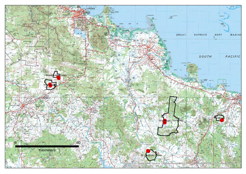
An updated version of this dataset is available at https://eatlas.org.au/data/uuid/38b496a3-3fba-42e7-b904-902f68040c85 Key Gully monitoring localities (headcuts and monitoring instrumentation) and outlines of the properties within which they are located. The data in presented in this metadata are part of a larger collection and are intended to be viewed in the context of the project. For further information on the project, view the parent metadata record: Demonstration and evaluation of gully remediation on downstream water quality and agricultural production in GBR rangelands (NESP TWQ 2.1.4, CSIRO) Methods: Key Gully Localities were extracted from the 2017 or 2018 RTK GPS surveys for each gully site (see Site_Configuration_and_Survey). Property Boundaries were generated by extracting polygons from the 2016 Digital Cadastre Database (DCDB) and simplifying to a single polygon. Area in hectares was calculated and appended to polygon attributes. KMZ’s are exported version of the original ArcGIS shapefiles Format: This data collection consists of two shapefiles (zipped) and two equivalent KMZ files with the following names: NESP_Gully_Key_localities Key gully localities include the RTK GP location of the instrumentation and the RTK GPS location of the nickpoint in the gully headcut rim. NESP_Gully_Property_Boundaries Boundaries for the properties on which the paired control/treatment gullies are located. Data Dictionary: Attributes for Property_Boundaries.shp include property NAME and the area in hectares (AREA_HA). Attributes for Key Locations include X,Y (MGA94 Z55) and Z (AHD) Timestamp associated when RTK surveyed Type- HEADCUT, INSTR Survey – type of survey and year, APPROX is best guess from Lidar or GoogleEarth Site_Code – short form code for sites where MIV = Minnievale MV = Meadowvale MW = Mount Wickham SB = Strathbogie VP = Virginia Park <T/C> - Treatment/Control Property – Full name of property Treat_type – Treatment or control References: Bartley, Rebecca; Hawdon, Aaron; Henderson, Anne; Wilkinson, Scott; Goodwin, Nicholas; Abbott, Brett; Baker, Brett; Matthews, Mel; Boadle, David; Jarihani, Ben (Abdollah). (2018) Quantifying the effectiveness of gully remediation on off-site water quality: preliminary results from demonstration sites in the Burdekin catchment (second wet season). RRRC: NESP and CSIRO. csiro:EP184204. Data Location: This dataset is filed in the eAtlas enduring data repository at: data\NESP2\2.1.4_Gully-remediation-effectiveness

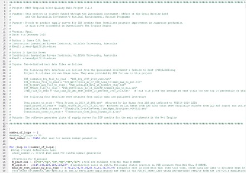
P2R.data.reader.v041220 with Header.R This is a block of R code written for NESP Tropical Water Quality Hub Project 3.1.6 The software uses data supplied from the Queensland Government’s Paddock to Reef (P2R) modelling system, and other publicly available data, to generate plots of supply curves for water quality credits in dissolved inorganic nitrogen (DIN) for the main catchments in the Wet Tropics. The aim of Project 3.1.6 was to compare the cost of supplying DIN credits from various sources with the prices that potential credit buyers would be willing to pay for those credits. This R-code estimates the minimum cost of supplying DIN credits via fertiliser practice change in sugarcane production in the main Wet Tropics catchments (Daintree, Mossman, Barron, Mulgrave-Russell, Johnstone, Tully, Murray and Herbert). Key data inputs on reductions in cane yield and reductions in DIN loss from 563 individual cane land management units[1] in the Wet Tropics are obtained from the Queensland Government’s Paddock to Reef (P2R) modelling program. Data on fertiliser cost, sugar prices, sugar content in cane, equipment cost and growers’ ‘transaction cost’ in engaging in water quality credit trading are obtained from public sources and the literature. Results are produced in the form of estimated supply curves for DIN credits from practice change in cane for the main Wet Tropics catchments. [1] The Queensland Government’s Paddock to Reef (P2R) modelling and monitoring program (The Australian and Queensland Governments, 2018) defines unique combinations of soil type, soil permeability, climate zone and sub-catchment in sugarcane land in the Wet Tropics catchments as separate cane ‘management units’. Methods: The Queensland Government’s Paddock to Reef (P2R) modelling and monitoring program (The Australian and Queensland Governments, 2018) defines unique combinations of soil type, soil permeability, climate zone and sub-catchment in sugarcane land in the Wet Tropics catchments as separate cane ‘management units’. P2R’s mapping produces 563 separate cane management units for which full cane yield and DIN loss predictions are available over the time period 1987-2013. In Project 3.1.6, the minimum cost of supplying DIN credits from practice change in cane in the Wet Tropics at management unit resolution is calculated as the sum of the following four components: 1. Opportunity cost: the reduction in average annual farm gross margin that follows from a reduction in fertiliser application rate. Average farm gross margin is derived from average P2R-simulated cane yields over the period 1987-2013 (Fraser et al., 2013). Opportunity cost is calculated on an annual basis. 2. Compensation for increased exposure to risk of reduced yield: the average reduction in farm gross margin from years containing the top 10% of P2R-simulated yields over the period 1987-2013 that follows from a reduction in fertiliser application rate (Fraser et al., 2013). Compensation for increased exposure to risk is calculated on an annual basis. 3. Transition cost: the annualised cost of equipment purchases required to implement each step improvement in fertiliser practice. Transition cost data are drawn from van Grieken et al., (2019; Table 2, p.4), inflated to 2018AUD using the Reserve Bank of Australia’s inflation calculator (https://www.rba.gov.au/calculator/ ).Transition cost is annualised over the 6-year cane cycle at a discount rate of 7% per annum, to produce an annualised equivalent transition cost that is compatible with the annual timeframe over which opportunity cost and the compensation required for increased exposure to risk are calculated. 4. Transaction cost: the annualised cost of the resources, including time, that a landholder has to commit to learn about and engage with water quality credit trading. Transaction cost data are drawn from (Coggan et al., 2014; Table 5, p.512), inflated to 2018AUD using the Reserve Bank of Australia’s inflation calculator (https://www.rba.gov.au/calculator/ ).Transaction cost is annualised over a 6-year cane cycle at a discount rate of 7% per annum to produce an annualised equivalent transition cost that is compatible with the annual timeframe over which opportunity cost and the compensation required for increased exposure to risk are calculated. Each element of cost is calculated for each step change in fertiliser management practice in line with the Sugarcane Water Quality Risk Framework 2017-2022 (The Australian and Queensland Governments, n.d.)(https://www.reefplan.qld.gov.au/__data/assets/pdf_file/0036/78867/sugarcane-water-quality-risk-framework-2017-2022.pdf ) i.e. for successive step improvements in fertiliser management practice on the Sugarcane Water Quality Risk Framework – Practice Level D to Practice Level C, Practice Level C to Practice Level B etc. Estimates of transition cost and transaction cost vary depending on the size of the farm within which a management unit is located. These data were not available to Project 3.1.6, so management units are stochastically allocated to small, medium or large farms across multiple simulation loops. Within each stochastic allocation, the total land area allocated to the different size classes of farms is matched to within 1% of that reported by Sing and Barron (2014). The initial level of fertiliser practice is also allocated stochastically across management units to match the proportion of catchment land area managed under the different levels of fertiliser practice as reported in the 2017 and 2018 Reef Report Cards (Commonwealth of Australia and Queensland Government, 2018). For each step change in fertiliser management practice on each management unit, the cost incurred (the sum of opportunity cost, compensation required for exposure to increased risk, transition cost and transaction cost) and the reduction in DIN loss achieved (at the cane field and at End-of-Catchment) are recorded. (Management unit-specific DIN transport coefficients for DIN lost via the surface water pathway are provided by P2R modelling. A uniform DIN transport coefficient from the literature is used for DIN lost via deep drainage (after Webster et al., (2012), as cited in van Grieken et al., 2019; Sec 3.3, p.4). The supply curve for supply of DIN credits from a catchment is constructed by ordering practice change steps from management units in that catchment from the most cost-effective (i.e. lowest $/kgDIN @ EoC) to the least cost-effective (i.e. highest $/kgDIN @ EoC), and then plotting cumulative DIN reduction (kgDIN reduced @ EoC) vs cost-effectiveness ($/kgDIN @ EoC). See Figure 5.5 to 5.9 in the final report ( https://nesptropical.edu.au/wp-content/uploads/2021/01/NESP-TWQ-Project-3.1.6-Final-Report.pdf ). Format: This data delivery is presented as a block of R-code. The first few lines of the tab-delimited input data files are also included in the data delivery to illustrate the format and content of the input data. Datafiles containing P2R data cannot be included in the eAtlas archive because Project 3.1.6 does not hold the rights to these data. Data Dictionary: Data delivery comprises: R-code to generate DIN credit supply curves, plus input data files R-code file: P2R.data.reader.v041220 with Header.R Input data files: as tab-delimited text files Data from Paddock to Reef (P2R): file header only included P2R_combined_Avg_file_to_read = "P2R_Avg_1987_2013_wide.txt" P2R_DINLoss_file_to_read = "P2R_WetTropics_Av_of_DIN_Loss_trimmed_max_to_min.txt" P2R_Herbert_Avg_file_to_read = "P2R_Averaged_data_in_Herbert_only.txt" P2R_FWCane_file_to_read = "P2R_WetTropics_Av_of_CaneFW_trimmed_max_to_min.txt" CVaR_file_to_read = "P2R_CVaR_by_DMU_Best_Worst_10_percent_1987_2013.txt" Publicly available data, compiled by NESP Project 3.1.6 Urea_prices_to_read = "Urea_Prices_in_2018_19_AUD.txt" Sugar_prices_to_read = "Sugar_Prices_in_2018_19_AUD.txt" Transition_costs_to_read = "Transition_Costs_between_Cane_Mgmt_Practices_v040520.txt" Transaction_costs_to_read = "Transaction_Cost_Data_Coggan_2014.txt" References: Coggan, A., van Grieken, M., Boullier, A., Jardi, X., 2014. Private transaction costs of participation in water quality improvement programs for Australia’s Great Barrier Reef: Extent, causes and policy implications. Aust. J. Agric. Resour. Econ. 59, 499–517. https://doi.org/10.1111/1467-8489.12077 Commonwealth of Australia and Queensland Government, 2018. Agricultural Land Management Practice Adoption Results: Reef Water Quality Report Card 2017 and 2018. Fraser, G., Shaw, M., Silburn, M., 2013. Paddock to Reef 2: Cane Paddock Scale Modelling – Wet Tropics Region. Sing, N., Barron, F., 2014. Management practice synthesis for the Wet Tropics region: A report prepared for the Wet Tropics Water Quality Improvement Plan. Terrain NRM, Innisfail. Terrain NRM, Innisfail. Queensland. The Australian and Queensland Governments, 2018. Paddock to Reef Integrated Monitoring, Modelling and Reporting Program 2017-2022: Summary. The Australian and Queensland Governments, n.d. Sugarcane water quality risk framework 2017-2022. van Grieken, M.E., Roebeling, P.C., Bohnet, I.C., Whitten, S.M., Webster, A.J., Poggio, M., Pannell, D., 2019. Adoption of agricultural management for Great Barrier Reef water quality improvement in heterogeneous farming communities. Agric. Syst. 170, 1–8. https://doi.org/10.1016/j.agsy.2018.12.003 Webster, A.J., Bartley, R., Armour, J.D., Brodie, J.E., Thorburn, P.J., 2012. Reducing dissolved inorganic nitrogen in surface runoff water from sugarcane production systems. Mar. Pollut. Bull. 65, 128–135. https://doi.org/10.1016/J.MARPOLBUL.2012.02.023 Data Location: This dataset is filed in the eAtlas enduring data repository at: data\nesp3\3.1.6_Exploring-WQ-trading\

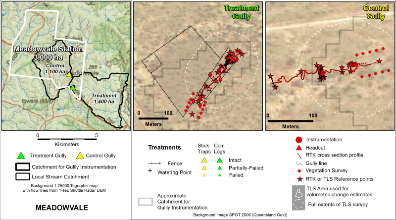
This dataset contains RTK GPS Data collected between April, 2017 and March, 2018 for 5 paired Control/Treatment gully sites being monitored as part of NESP Project 2.1.4 (Demonstration and evaluation of gully remediation on downstream water quality and agricultural production in GBR rangelands). The key question being asked is “is there measurable improvement in the erosion and water quality leaving remediated gully sites compared to sites left untreated?” The monitoring approach uses a modified BACI (Before after control impact) design. The data in presented in this metadata are part of a larger collection and are intended to be viewed in the context of the project. For further information on the project, view the parent metadata record: Demonstration and evaluation of gully remediation on downstream water quality and agricultural production in GBR rangelands (NESP TWQ 2.1.4, CSIRO). Monitoring of these sites is continuing as part of NESP TWQ Project 5.9. Any temporal extensions to this dataset will be linked to from this record. Methods: RTK (Real time kinematic) GPS system (Ashtech, ProMark 200), set with a tolerance of +/- 12mm in the horizontal plane and +/- 15mm in the vertical, was used to survey the monitored gullies. The initial location of the base station was determined using a 10-minute average. All permanent infrastructure such as survey markers, fences, and instrumentation. Gully features such as headcut rims, long sections and cross sections (at key locations such as near instrumentation) were captured. Raw GPS data files were converted to text, imported to Excel for attribute assignments, and then imported to ArcGIS for conversion to shapefile format. Format: This data collection consists of 5 zip files (one for each paired gully monitoring site). Zip files are named according to the property on which they are located. Each zip file contains two shapefiles with detailed RTK GPS survey data from either 2017 or 2018 for the Control and Treatment gullies. Survey point types include Reference markers, gully cross sections, long sections and the gully headcut. Data Dictionary: Attributes for each point include Easting (E) and Northing (N) location info (MGA94 Z55, AHD), descriptive text (Comment), horizontal accuracy (HRMS), vertical accuracy (VRMS), RTK Fix or Float status (STATUS), Number of satellites (SATS), 3D position dilution of precision (PDOP), horizontal dilution of precision (HDOP), Vertical dilution of precision (VDOP), time and date of survey point(Timestamp), and Point type (Type). More information on Dilution of Precision can be found here: https://en.wikipedia.org/wiki/Dilution_of_precision_(navigation) Point Types include REF and BASEREF - Reference markers include permanent survey markers XSREF - Cross Section Transect markers VEGREF - vegetation transect markers STRUCTREF) - Structure markers INSTRREF - location of instrumentation TLSREF - Laser scanner permanent markers gully cross sections (XS) LS - long sections RIM - headcut rim RIMNICK - headcut nickpoint Site_Code used for file names is as follows: MIV = Minnievale MV = Meadowvale MW = Mount Wickham SB = Strathbogie VP = Virginia Park <T/C> - Treatment/Control References: Bartley, Rebecca; Hawdon, Aaron; Henderson, Anne; Wilkinson, Scott; Goodwin, Nicholas; Abbott, Brett; Baker, Brett; Matthews, Mel; Boadle, David; Jarihani, Ben (Abdollah). Quantifying the effectiveness of gully remediation on off-site water quality: preliminary results from demonstration sites in the Burdekin catchment (second wet season). RRRC: NESP and CSIRO; 2018. csiro:EP184204. Data Location: This dataset is filed in the eAtlas enduring data repository at: data\nesp2\2.1.4 Gully-remediation-effectiveness

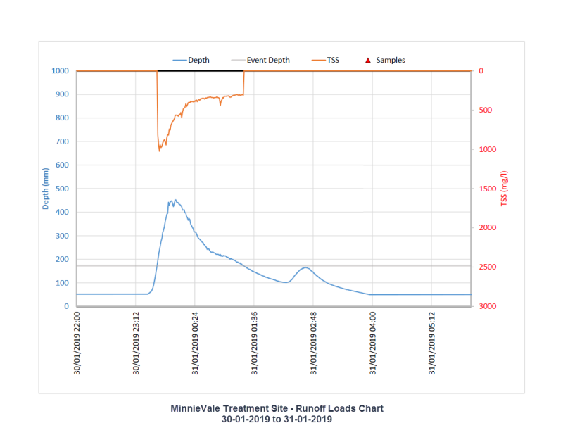
This dataset contains preliminary estimates of discharge and loads (Total suspended sediment and total nitrogen) based on monitoring data collected for the NESP Project 2.1.4 Demonstration and evaluation of gully remediation on downstream water quality and agricultural production in GBR rangelands. The data in presented in this metadata are part of a larger collection and are intended to be viewed in the context of the project. For further information on the project, view the parent metadata record: Demonstration and evaluation of gully remediation on downstream water quality and agricultural production in GBR rangelands (NESP TWQ 2.1.4, CSIRO). Monitoring of these sites is continuing as part of NESP TWQ Project 5.9. Any temporal extensions to this dataset will be linked to from this record. Methods: To estimate loads of suspended sediment (TSS) and total nitrogen (TN) the following steps were undertaken: (1) Depth, velocity and RTK surveyed cross-sectional area data were used to generate a stage-discharge rating curve for each site; (2) Linear relationships between TSS and TN sample concentrations and coincident turbidity data were derived for all sites (Table 6). Turbidity data was not used when (i) the instrument exceeded the instrument calibration threshold; (ii) turbidity sensor readings were erroneous due to damage or sensor malfunction, or when the sensors were buried. These relationships allowed for estimation of TSS and N from turbidity. When there was no turbidity data (due to sensor issues or instrument burial), TSS and TN concentrations were infilled using sample interpolation. (3) Total suspended sediment (TSS) and total nitrogen (TN) loads were then generated for each event and each water year (generally Nov to April) by multiplying discharge by concentration. (4) For all sites flow weighted annual average mean concentrations (FWAAC) were generated by dividing the annual load by annual runoff. This provided a quick visual assessment of the relative change in concentration between sites. (5) For some sites (i.e. Mt Wickham) event mean concentrations (EMCs) were generated for individual events by dividing the event load by event runoff. This provided a flow weighted mean concentration for each event. The event mean concentration (EMC) value for each event and year was calculated using mass of the sediment (in tonnes) divided by the runoff volume (in ML) during the time interval (T) (after Kim et al., 2004). Limitations of the Data: This dataset contains Water Quality monitoring data collected at these gully sites for the three reporting wet seasons spanning June-July 2016-2017, 2017-2018 and 2018-2019. During this study, the project had challenges with (i) sensor malfunctions (ii) sensor burial and re-scour (iii) sensors being damaged by moving objects (iv) green ant nests in sensors and (v) wires chewed by livestock. In addition sampling error or uncertainty in the discharge and load calculations can be high in semi-arid systems (Kuhnert et al., 2012). Consequently, all runoff and loads estimates are considered preliminary and will likely change in subsequent reporting years. Format: This data collection consists of 5 zip files (one for each paired gully monitoring site). Zip files are named according to the property on which they are located. Each zip file contains eight to twelve MS Excel spreadsheets representing daily and annual discharge and load estimates for both the Control and Treatment gully sites. MS Excel files contain tabs representing the following: SETUP – contains the site specific parameters used to estimate discharge and loads such as catchment size, location of instruments relative to depth sensor or gully cross section, discharge rating curve, and constituent-turbidity relationship SUMMARY – provides annual totals for rainfall, runoff, and loads, daily rainfall runoff chart, summary tables of rainfall and runoff events. RUNOFF_LOADS_CHART – chart of timeseries of depth, event depth, TSS or N concentration (as estimate from turbidity) and sample concentration - used to check for issues with depth or turbidity when interpreting annual or daily totals DAILY_SUMMARY_ALL_DATES – for generating daily rainfall, runoff and load estimates SAMPLES – list of sample values relevant to loads sheet period for cross checking against turbidity relationship RUNOFF LADS CALCS ALL TIMESTEP - raw Stream data with associated instantaneous calculations of discharge and loads RAIN AT GAUGE – rainfall timeseries from site (or closest) gauge RAIN USED FOR AVERAGING – if catchment is large, a second rain gauge may be used for averaging (not usually for gullies) Data Dictionary: Column headings used in the Excel spreadsheets: Timestamp – time in AEST (+10GMT) Depth – Depth of flow above depth sensor in millimetres, Depth sensor was level with gully bed at time of installation. Turbidity or Turb – turbidity in units of NTU (note that the Turbidity and velocity sensors are mounted above the depth sensor by 100 mm or more). Rainfall – rainfall in millimetres Discharge – discharge as either a rate or a total volume of water Runoff – discharge divided by catchment area Sample – Sample Number as submitted to Lab TSS / N = Total Suspended Sediment / Total Nitrogen Site_Code used for file names is as follows: MIV = Minnievale MV = Meadowvale MW = Mount Wickham SB = Strathbogie VP = Virginia Park <T/C> - Treatment/Control Note: SBT is now the Strathbogie Control site SBC (to 2018) and SBT2 (after 2018) is now the Strathbogie Treatment site References: Bartley, Rebecca; Hawdon, Aaron; Henderson, Anne; Wilkinson, Scott; Goodwin, Nicholas; Abbott, Brett; Baker, Brett; Matthews, Mel; Boadle, David; Jarihani, Ben (Abdollah). (2018) Quantifying the effectiveness of gully remediation on off-site water quality: preliminary results from demonstration sites in the Burdekin catchment (second wet season). RRRC: NESP and CSIRO. csiro:EP184204. Baker, B., Hawdon, A. and Bartley, R., 2016. Gully remediation sites: water quality monitoring procedures, CSIRO Land and Water, Australia. eAtlas Visualisation The visualisation presented on the eAtlas maps is a derived product of the summary data found within this data collection. A summary dataset was created using information presented on each spreadsheet [Water-Year, Site, Catchment Area, Rainfall, Runoff, %Runoff, Total TSS Load, Average TSS from time series, Total N Yield, N Loss, Average B from timeseries]. Two additional columns were added to the core information: data infill as referenced in the spreadsheets, has been represented in column 'Contains_Infilled_Data' noting Y or N; column 'Treatment_Control' was added to the summary dataset to aid visual representation, where treatment 'T' and control 'C' sites clearly identified. Data Location: This dataset is filed in the eAtlas enduring data repository at: data\nesp2\2.1.4_Gully-remediation-effectiveness

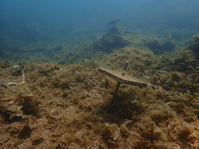
This dataset consists of monitoring data from macroalgae removal and larval seeding experiments in Florence and Arthur Bay at Magnetic Island, Queensland, Australia, collected between 2018-2020. There were twelve 5x5m permanent plots in each bay; three with macroalgae removal only, three with larval seeding only, three with macroalgae removal and larval seeding and three control plots. These data include: - Stationary point count fish survey data - Photo quadrats - Coral recruitment to settlement tiles - Macroalgae frond height, holdfast presence and biomass removed **This dataset is currently under embargo. The first phase of the project (2018-2019) was macroalgae removal only, with six permanent plots in each bay (three removal, and three controls). The second phase, beginning in July 2019, included six additional plots in each bay (n=12 plots per bay) and an additional experimental treatment in Arthur Bay only, where settlement-ready coral larvae were added to six of the plots per bay (n=3 plots per treatment). In Florence Bay, upon addition of the six new plots, the six original plots were re-assigned within the algal removal treatments (n=6 plots per treatment). Original plots in Arthur Bay maintained their designation of removal / non-removal, and these designations were then superimposed with larvae / no larvae. Methods: - Fish surveys: Fifteen-minute stationary point counts (SPC) with all fish present recorded, followed by a cryptic crawl (CC) consisting of five-minute search for additional species within the plot. Data was collected from March 2019 to February 2020 (4 surveys). - Photos: Three quadrats in each bay were randomly assigned for macroalgae removal and the remaining three were left untouched, representing control quadrats. Each quadrat was divided into 25 squares (1x1 m) using transect tapes, which form a gridline formation, and these squares were photographed using a digital camera at a distance of approximately 1 m above the region of interest at each survey time point. Reef benthic monitoring photographs were obtained at all quadrats (n=12) prior to macroalgae removal as a baseline in October 2018 and were recorded again immediately after manual removal of macroalgae from three of the quadrats in each bay (n=6). Four subsequent reef monitoring photograph surveys were conducted between November 2018 and May 2019. A total of 1650 photographs were obtained for this survey period. - Natural Recruits: Within the twenty-four 5x5m plots, three replicate 1x1m quadrats were haphazardly placed. All coral recruits up to 4cm were counted within the 1m2 quadrat and categorised as “branching” or “other” morphology. Recruits were also measured and categorised by diameter (i.e. 0-1cm, 1-2cm, 2-3cm, and 3-4cm). For treatment (i.e. algal removal) plots, this process was completed both before and after algal removal. - Recruit and lab reared tiles: Terra cotta tiles were used as a proxy for bare substrate, and were installed on the reef approximately 6 weeks prior to the mass spawning event in 2018 and 2019. Following the 2018 spawning, tiles were removed at two time points – February and March 2019 – to assess recruitment success and growth between control and removal plots. Upon removal, tiles were soaked for 48 hours in a 5% sodium hypochlorite solution. Coral skeletons were counted, measured, and photographed using a Nikon SMZ745T photo-microscope. Prior to the 2019 spawning, twenty adult coral colonies were removed from Horseshoe Bay, Magnetic Island and used as broodstock. These twenty colonies were maintained in aquaria at the National Sea Simulator at AIMS. Their spawn was collected, allowed to fertilise, and cultured in aquaria for 5 days. The competent larvae were released into specialised underwater tents into each of six treatment plots (3 with algal removal, 3 without) in Arthur Bay. An initial settlement check was performed by removing the settlement tiles and examining them under a microscope, counting all recruits, and placing the tiles back into the plots. Recruit counts were repeated in February and October 2020. - Macroalgae: Three 1x1m squares were haphazardly selected within each plot and the total number of macroalgae holdfasts recorded by divers. Algal height was measured for 10 algal fronds (from holdfast to end of frond). Biomass was the wet weight of algae removed from the removal plots. Limitations of the data: - Fish: Surveys were only done during daylight hours, so nocturnal fish are likely to have been missed, visibility was low at times making it harder to see fish, cryptic fishes are often missed during visual surveys. - Photo quadrats: Algae canopy can make it difficult to estimate benthic cover, ID challenges in general, low visibility makes it challenging to get clear photos. - Recruits: Bleaching method doesn’t allow to see if a recruit was alive when sampled; settlement tiles are not exact analogues to natural reef environment; some tiles were lost or tampered with. - Algae: Macroalgae were not identified to species level, it can be hard to define what a holdfast is. Format: This dataset consists of four spreadsheets datasets associated with the ecology and community composition of the experiments. 1_Fish_Data Fish community data from underwater surveys 2_Photo_Quadrats Photos showing benthic cover (coral, macroalgae etc.) within experimental plots 4_Natural_Recruits Coral recruits to tiles within experimental plots without larval seeding 5_Recruit&Lab-reared_Tiles Coral recruits to tiles for the larvae seeding experiments 6_Macroalgae Macroalgae frond height, number of holdfasts and biomass of removed macroalgae Data Dictionary: Fish surveys: File: Fish - macroalgae removal experiments magnetic island.xlsx [2 datasheets: Stationary Point Count (SPC) & Cryptic Crawl (CC)] - Date: Date of survey - Time: Survey start time - Bay: Two sites on Magnetic Island were surveyed - Arthur and Florence Bays - Plot: Fixed plot number surveyed at each of 2 sites - Treatment: Control, Removal only, Larvae, Removal and larvae - ID: sample/quadrat photo ID - Visibility (m): water visibility assessed by diver at start of dive - Species: Fish species observed - Count: Total number of fish of each species observed - Observer: Name of diver recording fish data Natural Recruits: *Note that this part of monitoring commenced in the “Study” phase, so no pilot data exists (nor does the column specifying study phase) File name: Recruits.csv - LOCATION: Two sites on Magnetic Island - Arthur and Florence Bays - PLOT: Fixed plot number surveyed at each of 2 sites - DATE: Date of survey - QUADRAT: Replicate 1x1m square quadrat within each experimental plot - TREATMENT: Treatment, macroalgae removal, larval enhancement, both or none. - PRE-POST: when the survey was conducted, either pre- or post-removal of algae - SIZE: categories of recruit diameter where 1=0-1cm; 2 = 1-2cm; 3 = 2-3cm, 4 = 3-4cm - MORPHOLOGY - COUNT: number of coral recruits observed - OBSERVER: The person who made the observation Lab-reared recruits: File name: LabRearedRecruits.xlsx [2 datasheets: Treatment & Control] - Sort: Individual identifier - Plot: Plot number - Treatment: Experimental treatment - Tile: Tile number - Surface: side of the tile where recruits were counted - Acroporidae: Number of recruits from the family Acroporidae - Total per tile: Total number of coral recruits per tile - Mean per tile plot: Mean number of coral recruits per tile within a plot - Mean per tile: Mean number of coral recruits per tile - Pocilloporidae: Number of recruits from the family Pocilloporida - Others: Number of coral recruits from other families Macroalgae: File name: Holdfasts.csv - BAY Two sites on Magnetic Island - Arthur and Florence Bays - PLOT Fixed plot number surveyed at each of 2 sites - HOLDFASTS The number of Sargassum holdfasts counted in each 1x1m replicate - DATE: date of survey - TREATMENT: Treatment of macroalgae removal, larval enhancement, both or none. - PRE/POST: when the survey was conducted, either pre- or post-removal of algae - OBSERVER: the person making the observation - STUDY-PHASE: either Pilot or Study. Pilot phase included 6 plots per bay, while Study phase included 12 plots per bay. Furthermore the plot treatment designations were changed in Florence Bay between Pilot and Study phases. - NOTES: miscellaneous text File name: Biomass.xlsx - BAY: Two sites on Magnetic Island – Arthur and Florence Bays - PLOT: Fixed plot number surveyed at each of 2 sites - DATE: date of survey - TREATMENT: Treatment of macroalgae removal, larval enhancement, both, or none - KG: Kilograms of wet weight macroalgae removed from each experimental plot, weighed to the nearest 0.1kg using fish scales. - OBSERVER: The person making the observation File name: Algae.csv - BAY: Two sites on Magnetic Island – Arthur and Florence Bays - PLOT: Fixed plot number surveyed at each of 2 sites - QUADRAT: Replicate 1x1m quadrat within each plot being surveyed. Three replicates per plot. - FROND: Replicate number of frond measurement, 1-10 - HEIGHT: Height of the algal frond from holdfast to frond tip, measured in cm. - DATE: Date of survey - TREATMENT: Treatment of macroalgae removal, larval enhancement, both, or none - PrePostRemoval: when the survey was conducted, either pre- or post-removal of algae - OBSERVER: the person making the observation - STUDY-PHASE: either Pilot or Study. Pilot phase included 6 plots per bay, while Study phase included 12 plots per bay. Furthermore the plot treatment designations were changed in Florence Bay between Pilot and Study phases. - NOTES: any miscellaneous text Data Location: This dataset is filed in the eAtlas enduring data repository at: data\nesp4\4.3_Best-practice-coral-restoration\

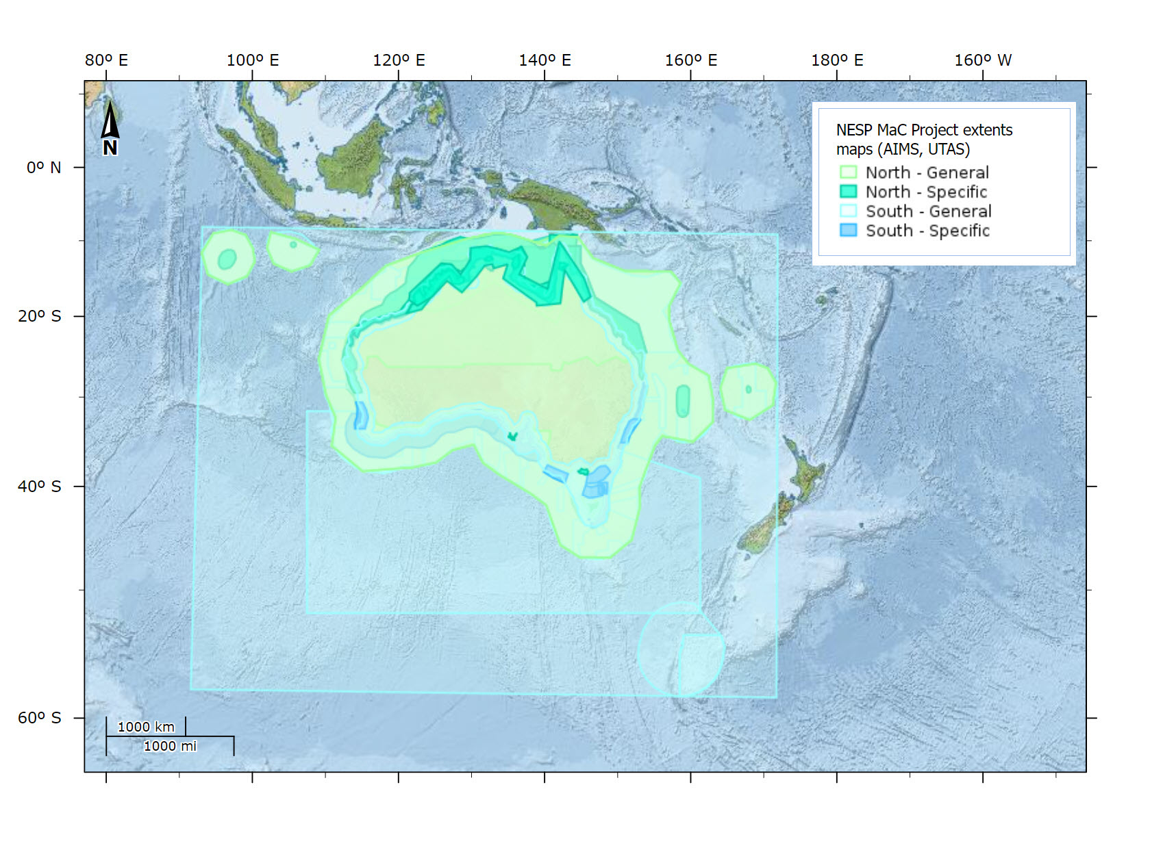
This dataset contains 63 shapefiles that represent the areas of relevance for each research project under the National Environmental Science Program Marine and Coastal Hub, northern and southern node projects for Rounds 1, 2 & 3. Methods: Each project map is developed using the following steps: 1. The project map was drawn based on the information provided in the research project proposals. 2. The map was refined based on feedback during the first data discussions with the project leader. 3. Where projects are finished most maps were updated based on the extents of datasets generated by the project and followup checks with the project leader. The area mapped includes on-ground activities of the project, but also where the outputs of the project are likely to be relevant. The maps were refined by project leads, by showing them the initial map developed from the proposal, then asking them "How would you change this map to better represent the area where your project is relevant?". In general, this would result in changes such as removing areas where they were no longer intending research to be, or trimming of the extents to better represent the habitats that are relevant. The project extent maps are intentionally low resolution (low number of polygon vertices), limiting the number of vertices 100s of points. This is to allow their easy integration into project metadata records and for presenting via interactive web maps and spatial searching. The goal of the maps was to define the project extent in a manner that was significantly more accurate than a bounding box, reducing the number of false positives generated from a spatial search. The geometry was intended to be simple enough that projects leaders could describe the locations verbally and the rough nature of the mapping made it clear that the regions of relevance are approximate. In some cases, boundaries were drawn manually using a low number of vertices, in the process adjusting them to be more relevant to the project. In others, high resolution GIS datasets (such as the EEZ, or the Australian coastline) were used, but simplified at a resolution of 5-10km to ensure an appopriate vertices count for the final polygon extent. Reference datasets were frequently used to make adjustments to the maps, for example maps of wetlands and rivers were used to better represent the inner boundary of projects that were relevant for wetlands. In general, the areas represented in the maps tend to show an area larger then the actual project activities, for example a project focusing on coastal restoration might include marine areas up to 50 km offshore and 50 km inshore. This buffering allows the coastline to be represented with a low number of verticies without leading to false negatives, where a project doesn't come up in a search because the area being searched is just outside the core area of a project. Limitations of the data: The areas represented in this data are intentionally low resolution. The polygon features from the various projects overlap significantly and thus many boundaries are hidden with default styling. This dataset is not a complete representation of the work being done by the NESP MaC projects as it was collected only 3 years into a 7 year program. Format of the data: The maps were drawn in QGIS using relevant reference layers and saved as shapefiles. These are then converted to GeoJSON or WKT (Well-known Text) and incorporated into the ISO19115-3 project metadata records in GeoNetwork. Updates to the map are made to the original shapefiles, and the metadata record subsequently updated. All projects are represented as a single multi-polygon. The multiple polygons was developed by merging of separate areas into a single multi-polygon. This was done to improve compatibility with web platforms, allowing easy conversion to GeoJSON and WKT. This dataset will be updated periodically as new NESP MaC projects are developed and as project progress and the map layers are improved. These updates will typically be annual. Data dictionary: NAME - Title of the layer PROJ - Project code of the project relating to the layer NODE - Whether the project is part of the Northern or Southern Nodes TITLE - Title of the project P_LEADER - Name of the Project leader and institution managing the project PROJ_LINK - Link to the project metadata MAP_DESC - Brief text description of the map area MAP_TYPE - Describes whether the map extent is a 'general' area of relevance for the project work, or 'specific' where there is on ground survey or sampling activities MOD_DATE - Last modification date to the individual map layer (prior to merging) Updates & Processing: These maps were created by eAtlas and IMAS Data Wranglers as part of the NESP MaC Data Management activities. As new project information is made available, the maps may be updated and republished. The update log will appear below with notes to indicate when individual project maps are updated: 20220626 - Dataset published (All shapefiles have MOD_DATE 20230626) Location of the data: This dataset is filed in the eAtlas enduring data repository at: data\\custodian\nesp-mac-3\AU_AIMS-UTAS_NESP-MaC_Project-extents-maps

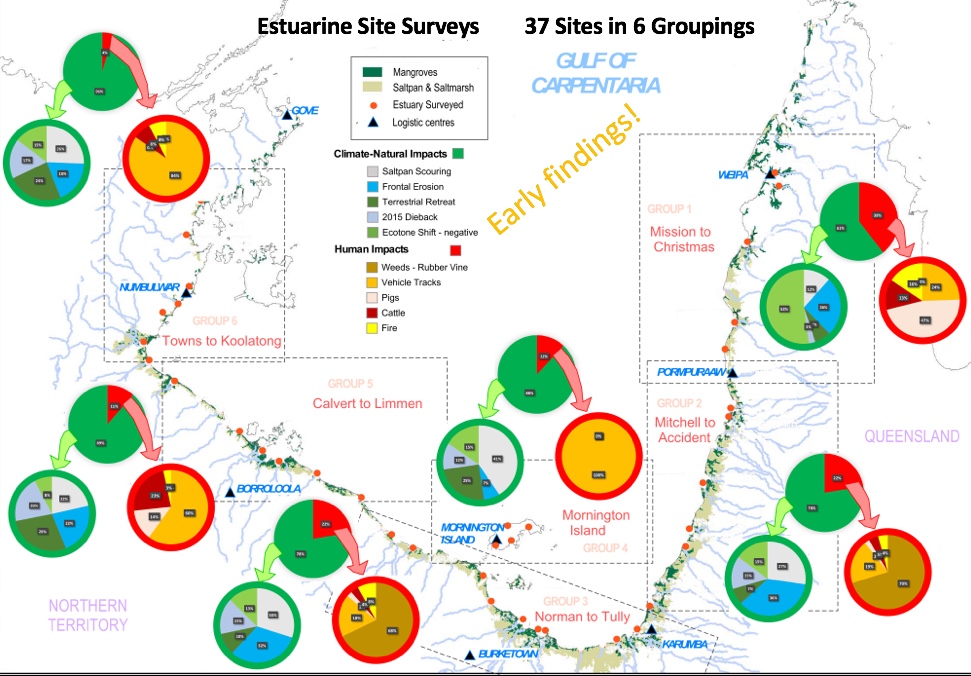
The major estuaries and their tidal wetlands of the Gulf of Carpentaria were impacted by mass dieback of mangroves in 2015-2016. To assess the full extent of the dieback and the major changes in the wetland areas, surveys in 2017 and 2019 were conducted along 31–37 major estuary mouths. Methods: The estuary surveys were conducted during aerial surveys using the same methods generally (see associated metadata record for more details: Gulf of Carpentaria Mangrove Aerial Shoreline Surveys 2017 & 2019 (NESP TWQ 4.13, JCU)). Shoreline edges were filmed and observations scored within a few kilometres of each estuary mouth. The observations recorded included a standard set of 10-20 features related to natural and human associated pressures like storm impacts, shoreline erosion, 2015 dieback of mangroves, fire damage, feral pig damage plus roads and buildings. Observations were summarised for each factor based on extent and severity scores to provide respective rankings of influence. These observations were further linked to respective likely drivers like sea level rise, storm winds, rough seas, plus the human associated ones of fire, pigs and weeds. The surveys collected observational data to classify the state, condition and health of the shoreline using criteria: 1. Driver type: list the drivers of change observed 2. Indicator: the indicator observed 3. Habitat: listing of the tidal wetland habitats affected 4. Extent: estimate the proportion of the tidal wetland affected 5. Severity: estimate severity of impact – time to natural recovery and effect on ecosystem function/structure 6. Time frame: when did the impact occur 7. Observations: notes and other comments These strategies were used to evaluate habitat condition associated with particular drivers, as well as providing an evaluation of local and national management priorities. The follow criteria were used to score the extent, severity and time frame (where applicable) for the criteria: Variable: Extent of impact on the tidal wetlands – The extent of tidal wetlands impacted determined by the proportional area showing impact. Impact extent assessment scoring criteria: 1. 1 – 10% 2. 10 – 30% - around 25% 3. 30 – 60% - around 50% 4. 60 – 90 % - around 75% 5. >90% Assessment metric: Extent score – extent of impact in the tidal wetlands Variable: Severity of impact on tidal wetland area – the severity of tidal wetlands impacted as determined by the degradation state observed. Impact severity assessment scoring criteria: 1. None – present but no observable effect 2. Minor – recovery within less than one year 3. Moderate – recovery over 1 – 2 years 4. Major – recovery over 2 – 10 years 5. Severe – recovery unlikely – collapse/replace Assessment metric: Severity score – severity of impact in the tidal wetlands Variable: Time frame of the impact on tidal wetland area – The timing of the impact on tidal wetlands as determined by the recovery potential observed. Impact time frame Assessment scoring criteria: 1. No observable effect, but potentially so 2. Current – now 3. Recent – less than 2 years ago 4. 4. Old – 2- 10 years ago 5. Very old - >10 years Assessment metric: Time frame score – time of occurrence of impact affecting tidal wetland area. Limitations of the data: Format of the data: This data consists of the survey assessment sheets from each estuary (xlsx) plus summary spreadsheets for each survey year. Each survey assessment sheet presents the original scores for Extent and Severity for each of the variables, as well as the calculations for respective rankings of influence. Note - The rankings of influence was used for the basis of the map visualisation by eAtlas, presenting the combined summary for each survey year as a shapefile. Data dictionary: 2019 Gulf of Carpentaria Tidal Wetland Threat Assessment Sheets: The extent, severity, time frame, restoration potential and other observations were collected for each of the following variables: Human Related Variable Driver Type: Indicator / Habitat Structure Loss: rock walls, wharf, ramps, roads / any zone Direct Loss: clearing, dead trees, landfill / any zone Altered Hydrology: bunds, drains, impoundments / higher zones mostly Encroachment: no buffer, cut-off flows / upper edge zone Access Tracks: wheel tracks, foot paths / Salt pans + high tide margin Stock Impacts: cattle, horses, goats – tracks / Salt pans + high tide margin Feral Damage: pigs, wallows, digging and tracks / Salt pan mangrove + freshwater wetlands Pollutant impact: oil spill, scum, dump, dieback / any zone Nutrient Excess: enhanced growth, expansion / any zone Fire Scorch: burnt vegetation - grass, dieback, blackened / upper margin - fringing zone Weed Smother: smothering weeds present / Beach ridge veg - mangrove upper edges Climate-natural Variable Driver Type: Indicator / Habitat Storm Damage: broken stems, damaged canopies, dead trees / mangrove closed canopies Shoreline erosion: fallen trees, steep bank, dieback / seaward + main channel edge stands of mangroves Root Burial: dead trees, burying sediments /shoreline and sea edge mangroves Inner Fringe Collapse: patchy dieback, canopy gaps / waters edge canopies Bank Erosion: channel edges eroded, fallen trees, steep / lower estuary banks Pan Scouring: upper pan, eroded edges, sheet erosion / upper salt pans Ecotone Shift -ve: dead trees pan edges / saltpan – mangrove Ecotone Shift +ve: new growth – seedlings, saplings / saltpan – mangrove Depositional gain: new growth – seedlings, saplings / waters edge margins Terretrial Retreat: dead terrestrial edge trees, eroded edge /terrestrial fringe Light gaps: dead trees, circular patch / mangrove closed canopies Altered hydrology: impounded, ponded water, dead trees /shoreline and sea edge mangroves 2015 Dieback: dead trees on back front edge / rear of mangrove front 2017 Gulf of Carpentaria Tidal Wetland Threat Assessment Sheets: Driver Type: Indicator / Habitat Pigs: wallows, pigs and tracks / inner mangrove + freshwater wetlands Fire: burnt vegetation – grass / Terrestrial margin - fringing mangroves Vehicle tracks: wheel tracks / Salt pans + high tide edge Cattle: cattle and tracks / Salt pans + high tide edge Weeds: weed species present / Beach ridge veg. / to mangrove upper edges 2015 Dieback: dead trees on pan edges / mangrove closed canopies Ecotone Shift: dead trees on pan edges / AM + Ceriops closed canopies Terretrial Retreat: dead terrestrial edge trees / Terrestrial fringe Saltpan scouring: eroded edges – escarpments / upper saltpans Light gaps: dead trees in a small circular patch / mangrove closed canopies Storm Damage: damaged canopies, dead trees / Mangrove closed canopies Depositional gain: new growth - seedlings. Saplings / waters edge margins Shoreline erosion: inner fringe collapse / seaward + main channel edge stands of mangroves Bank Erosion: channel edges eroded / lower estuary banks Altered hydrology: impounded, ponded water, dead trees / shoreline and sea edge mangroves Root Burial: dead trees and mobile sediments / shoreline and sea edge mangroves Note in some cases similar terminology was used for the same attribute for the different survey years, i.e. Access Tracks = Vehicle tracks, Stock impacts = cattle, Feral Damage = pigs. Data Dictionary - Shapefile Attributes Shapefile Attributes / Data Attribute: Description CATCHMENT/CATCHMENT: Catchment name. Estuaries are grouped in catchment areas described in the CSIRO Northern Australia Sustainable Project [CSIRO (2009) Water in the Gulf of Carpentaria Drainage Division. A report to the Australian Government from the CSIRO Northern Australia Sustainable Yields Project. CSIRO Water for a Healthy Country Flagship, Australia. xl + 479pp] SITE_NO/SITE_NO Number allocated to the site NAME/LOCATION_NAME: Location name REPEAT SURVEY/REPEAT SURVEY: whether the survey was repeated in 2019 (Y) or not (N) LATITUDE/LATITUDE: Latitude of the survey location. Coordinates mark the location of each estuary mouth. LONGITUDE/LONGITUDE: Longitude of the survey location. Coordinates mark the location of each estuary mouth. MANGROVE_S/MANGROVE_SPP_NO: Number of observed mangrove species for the location. S19-HUMAN/HUMAN_ISSUES: Total score of all Human threat issues for the 2019 survey assessment. Indicates the combined entent and severity scores across all the human issues and gives an idea of which areas are most impacted for this category. S19-CLIMATE/CLIMATE _ISSUES: Total score of all Climate threat issues for the 2019 survey assessment. Indicates the combined entent and severity scores across all the human issues and gives an idea of which areas are most impacted for this category. S19_S_LOSS/2019_STRUCTURE_LOSS Rock walls, wharf, ramps, roads found on any habitat zone. Extent and severity were assessed according to fixed criteria, and the Extent*Severity summary score combined shows the respective rankings of influence. S19_D_LOSS/2019_DIRECT_LOSS: Clearing, dead trees, landfill found on any habitat zone. Extent and severity were assessed according to fixed criteria, and the Extent*Severity summary score combined shows the respective rankings of influence. S19_ALT_HY/2019_ALTERED_HYDROLOGY: Bunds, drains, impoundments on the higher zones mostly. Extent and severity were assessed according to fixed criteria, and the Extent*Severity summary score combined shows the respective rankings of influence. S19_ENCROA/2019_ENCROACHMENT: No buffer, cut-off flows on the upper edge habitat zone. Extent and severity were assessed according to fixed criteria, and the Extent*Severity summary score combined shows the respective rankings of influence. S19_TRACKS/2019_ACCESS_TRACKS: Wheel tracks and/or foot paths on the Salt pans & high tide margin. Extent and severity were assessed according to fixed criteria, and the Extent*Severity summary score combined shows the respective rankings of influence. S19_STOCK/2019_STOCK_IMPACTS: Cattle, horse or goats tracks on the Salt pans & high tide margin. Extent and severity were assessed according to fixed criteria, and the Extent*Severity summary score combined shows the respective rankings of influence. S19_FERAL/2019_FERAL_DAMAGE: Pigs, wallows, digging and tracks on the Salt pan mangrove & freshwater wetlands. Extent and severity were assessed according to fixed criteria, and the Extent*Severity summary score combined shows the respective rankings of influence. S19_POLLUT/2019_POLLUTANT_IMPACT: Oil spill, scum, dump, dieback found in any habitat zone. Extent and severity were assessed according to fixed criteria, and the Extent*Severity summary score combined shows the respective rankings of influence. S19_NUTRI/2019_NUTRIENT_EXCESS: Enhanced growth, expansion in any habitat zone. Extent and severity were assessed according to fixed criteria, and the Extent*Severity summary score combined shows the respective rankings of influence. S19_FIRE/2019_FIRE_SCORCH: Burnt vegetation (grass, dieback, blackened / upper margin) on the fringing zone. Extent and severity were assessed according to fixed criteria, and the Extent*Severity summary score combined shows the respective rankings of influence. S19_WEED/2019_WEED_SMOTHER: Smothering weeds present on the beach ridge vegetation - mangrove upper edges. Extent and severity were assessed according to fixed criteria, and the Extent*Severity summary score combined shows the respective rankings of influence. S19_STORM/2019_STORM_DAMAGE: Broken stems, damaged canopies or dead trees in the mangrove closed canopies. Extent and severity were assessed according to fixed criteria, and the Extent*Severity summary score combined shows the respective rankings of influence. S19_S_EROS/2019_SHORELINE_EROSION: Fallen trees, steep bank, dieback at seaward and main channel edge stands of mangroves. Extent and severity were assessed according to fixed criteria, and the Extent*Severity summary score combined shows the respective rankings of influence. S19_ROOT_B/2019_ROOT_BURIAL: Dead trees and burying sediments on the shoreline and sea edge mangroves. Extent and severity were assessed according to fixed criteria, and the Extent*Severity summary score combined shows the respective rankings of influence. S19_FRINGE/2019_INNER_FRINGE_COLLAPSE: Patchy dieback, canopy gaps at thewaters edge canopies. Extent and severity were assessed according to fixed criteria, and the Extent*Severity summary score combined shows the respective rankings of influence. S19_B_EROS/2019_BANK_EROSION: Channel edges eroded, fallen trees, steep lower estuary banks. Extent and severity were assessed according to fixed criteria, and the Extent*Severity summary score combined shows the respective rankings of influence. S19_PAN_SC/2019_PAN_SCOURING: Upper pan, eroded edges and/or sheet erosion on the upper salt pans. Extent and severity were assessed according to fixed criteria, and the Extent*Severity summary score combined shows the respective rankings of influence. S19_NEG_ES/2019_NEG_ECOTONE_SHIFT: Dead trees pan edges on the saltpan – mangrove habitat. Extent and severity were assessed according to fixed criteria, and the Extent*Severity summary score combined shows the respective rankings of influence. S19_POS_ES/2019_POS_ECOTONE_SHIFT: New growth – seedlings or saplings on the saltpan – mangrove habitat. Extent and severity were assessed according to fixed criteria, and the Extent*Severity summary score combined shows the respective rankings of influence. S19_D_GAIN/2019_DESPOSITIONAL_GAIN: New growth – seedlings, saplings at the waters edge margins. Extent and severity were assessed according to fixed criteria, and the Extent*Severity summary score combined shows the respective rankings of influence. S19_TERRE/2019_TERRETRIAL_RETREAT: Dead terrestrial edge trees or eroded edge on the terrestrial fringe. Extent and severity were assessed according to fixed criteria, and the Extent*Severity summary score combined shows the respective rankings of influence. S19_L_GAPS/2019_LIGHT_GAPS: Dead trees or circular patch on mangrove closed canopies. Extent and severity were assessed according to fixed criteria, and the Extent*Severity summary score combined shows the respective rankings of influence. S19_ALT_HY/2019_ALTERED_HYDROLOGY: Bunds, drains, impoundments on the higher zones mostly. Extent and severity were assessed according to fixed criteria, and the Extent*Severity summary score combined shows the respective rankings of influence. S19_2015_D/2019_2015_DIEBACK: Dead trees on back front edge of the rear of mangrove front. Extent and severity were assessed according to fixed criteria, and the Extent*Severity summary score combined shows the respective rankings of influence. S17_TRACKS/2017_ACCESS_TRACKS: Wheel tracks and/or foot paths on the Salt pans & high tide margin. Extent and severity were assessed in the 2017 survey according to fixed criteria, and the Extent*Severity summary score combined shows the respective rankings of influence. S17_STOCK/2017_STOCK_IMPACTS: Cattle, horse or goats tracks on the Salt pans & high tide margin. Extent and severity were assessed according to fixed criteria, and the Extent*Severity summary score combined shows the respective rankings of influence. S17_FERAL/2017_FERAL_DAMAGE: Pigs, wallows, digging and tracks on the Salt pan mangrove & freshwater wetlands. Extent and severity were assessed according to fixed criteria, and the Extent*Severity summary score combined shows the respective rankings of influence. S17_FIRE/2017_FIRE_SCORCH: Burnt vegetation (grass, dieback, blackened / upper margin) on the fringing zone. Extent and severity were assessed according to fixed criteria, and the Extent*Severity summary score combined shows the respective rankings of influence. S17_WEED/2017_WEED_SMOTHER: Smothering weeds present on the beach ridge vegetation and mangrove upper edges. Extent and severity were assessed according to fixed criteria, and the Extent*Severity summary score combined shows the respective rankings of influence. S17_STORM/2017_STORM_DAMAGE: Broken stems, damaged canopies or dead trees in the mangrove closed canopies. Extent and severity were assessed according to fixed criteria, and the Extent*Severity summary score combined shows the respective rankings of influence. S17_S_EROS/2017_SHORELINE_EROSION: Fallen trees, steep bank, dieback at seaward and main channel edge stands of mangroves. Extent and severity were assessed according to fixed criteria, and the Extent*Severity summary score combined shows the respective rankings of influence. S17_ROOT_B/2017_ROOT_BURIAL: Dead trees and burying sediments on the shoreline and sea edge mangroves. Extent and severity were assessed according to fixed criteria, and the Extent*Severity summary score combined shows the respective rankings of influence. S17_B_EROS/2017_BANK_EROSION: Channel edges eroded, fallen trees, steep on the lower estuary banks. Extent and severity were assessed according to fixed criteria, and the Extent*Severity summary score combined shows the respective rankings of influence. S17_PAN_SC/2017_PAN_SCOURING: Upper pan, eroded edges and/or sheet erosion on the upper salt pans. Extent and severity were assessed according to fixed criteria, and the Extent*Severity summary score combined shows the respective rankings of influence. S17_NEG_ES/2017_NEG_ECOTONE_SHIFT: Dead trees pan edges on the saltpan – mangrove habitat. Extent and severity were assessed according to fixed criteria, and the Extent*Severity summary score combined shows the respective rankings of influence. S17_POS_ES/2017_POS_ECOTONE_SHIFT: New growth – seedlings or saplings on the saltpan – mangrove habitat. Extent and severity were assessed according to fixed criteria, and the Extent*Severity summary score combined shows the respective rankings of influence. S17_D_GAIN/2017_DESPOSITIONAL_GAIN: New growth – seedlings, saplings at the waters edge margins. Extent and severity were assessed according to fixed criteria, and the Extent*Severity summary score combined shows the respective rankings of influence. S17_TERRE/2017_TERRETRIAL_RETREAT: Dead terrestrial edge trees or eroded edge on the terrestrial fringe. Extent and severity were assessed according to fixed criteria, and the Extent*Severity summary score combined shows the respective rankings of influence. S17_L_GAPS/2017_LIGHT_GAPS: Dead trees or circular patch on mangrove closed canopies. Extent and severity were assessed according to fixed criteria, and the Extent*Severity summary score combined shows the respective rankings of influence. S17_ALT_HY/2017_ALTERED_HYDROLOGY: Impounded, ponded water or dead trees on the shoreline and sea edge mangroves - Extent and severity were assessed according to fixed criteria, and the Extent*Severity summary score combined shows the respective rankings of influence. S17_2015_D/2017_2015_DIEBACK: Dead trees on back front edge of the rear of mangrove front - Extent and severity were assessed according to fixed criteria, and the Extent*Severity summary score combined shows the respective rankings of influence. References: Duke N.C., Mackenzie J., Kovacs J., Staben G., Coles, R., Wood A., & Castle Y. (2020). Assessing the Gulf of Carpentaria mangrove dieback 2017–2019. Volume 1: Aerial surveys. James Cook University, Townsville, 226 pp. eAtlas Processing: The original data were provided as excel spreadsheets. No modifications to the underlying data were performed and the data package are provided as submitted. The mapping product was generated based on the workbook 'GULF_Threat_Summary #2.xlsx' particularly the '2017-2019' tab & '2019_Gulf Threats ALL' tab (Human_Issues & Climate_Issues data columns). These figures were copied to a new csv file and formatted to optimise visualisation on the map. Columns not recorded during the 2017 survey were removed from the dataset to reduce the scroll length when observing the table associated with each point. Descriptions presented here are derived from information from the final report by the eAtlas team. Location of the data: This dataset is filed in the eAtlas enduring data repository at: data\\custodian\4.13_Assessing-gulf-mangrove-dieback

Vegetation and Elevation surveys were conducted at four sites in the Gulf of Carpenteria to provided crucial validation of observations made from aerial surveys and provided further significant insights of the impacts and subsequent changes that occurred across the Gulf coastline up to late 2019. Field studies primarily focused on shoreline fringing stands dominated by the Grey Mangrove Avicennia marina var. eucalyptifolia. A total of eight transects, perpendicular to the shoreline were established at four shoreline sites across the Gulf of Carpentaria. These included matched pairs for each of two severity levels of 90%–100% and 60%–80% dieback of mangrove fringes. A series of profile transects were established and measured from the landward edge to the sea edge of mangroves. Transects were run from a highwater point at the head, directly towards the sea edge. This method captured common reference elevation levels for all sites while maximising coverage of the entire elevation range of the tidal wetland (mangroves plus tidal saltpan and saltmarsh vegetation), from approximately highest astronomical tide levels (~HAT) at the head, to approximately mean sea level (~MSL) at the seaward edge of living mangrove trees. On ground surveys consisted of two components: a) elevation measures from HAT (highest astronomical height – defined by the highwater mark) to MSL (mean sea level – defined by the seaward mangrove edge); and b) vegetation species, structure and density for mangrove and saltmarsh species present along with observations of condition and being likely 2015 dieback. The latter condition was determined from vegetative degradation states of mangrove trees, and as seen in satellite imagery mapping. Methods: Locations: The field studies started with the two locations in Queensland during 4–10 August 2018 and then moved onto those in the Northern Territory during 11–17 October 2018. A total of eight transects, perpendicular to the shoreline were established at the four shoreline sites across the Gulf of Carpentaria. Limmen – Roper region (NT) - 1A with 90% - 100 % dieback - 1B with 60% - 80% dieback Mule - Roper region (NT) - 2B with 90% - 100 % dieback - 2A with 60% - 80% dieback Karumba - SE Gulf (QLD) - 4A with 90% - 100 % dieback - 4B with 60% - 80% dieback Mitchell north - W Cape (QLD) - 5A with 90% - 100 % dieback - 5D with 60% - 80% dieback Transect Set Up Summary: Each transect was based or anchored at the observed nominal Highest Astronomical Tide (~HAT) level of the highwater benchmark at each transect ‘head’, via the beach wash zones indicative of the highest reach of tidal waters. A second reference position at the sea edge of mangroves was taken as a proxy relative to mean sea level (~MSL). The location of the head position was chosen so that a straight line transect could be taken to the fringing mangrove stand, and to the sea edge at the proxy position of mean sea level (~MSL). Three additional ‘internal’ ecotone position markers between ~HAT and ~MSL of the tidal wetland zone were recorded for each transect, including the landward fringing mangrove to the saltpan–saltmarsh position (M1-lower); the lower elevation limit of saltpan–saltmarsh bordering the upper dieback mangrove edge (M2-upper); and the lower elevation limit of mangrove dieback (M2-dead/live). Further details about the transect set up can be found in the final report volume 2 (Duke et al, 2020). Surveys: Long plots were used to describe and quantify mangrove and saltmarsh vegetation along each transect. The long plot method allowed the plot width to be adjusted during the survey depending on stem density of particular sections along the transect - where there were closely spaced trees, plots were narrower (<2 m wide) than where trees were larger and further apart (>2 m wide). Elevation levels were recorded at 20–30 m intervals or more frequently where there were otable changes in topography or there were notable changes in vegetation type and condition. Levels were made using a Topcon construction surveyors rotating laser and staff. Where it was necessary to relocate the laser instrument, additional reference points were taken for each transition point providing offset measures to link each series of measurements. Elevation levels were recorded all the way from the head marker to the sea edge amongst or just beyond the last trees. Vegetation was scored for species, stem diameter, height, condition as well as distance along the transect and distance left or right of the measuring tape. Trees were scored in 30 m sections within a fixed distance from the measuring tape depending on stand density. The width was mostly set at two metres, but on occasion, this was reduced to one metre or up to four metres wide as necessary. Along each transect, at each 30-metre interval or at ecotone points, photographs were taken at four square directions to the transect line – towards the sea, 90 degrees to the right, back towards the ‘head’ and 90 degrees to the left. At these same points, canopy photos were taken using a camera with a fisheye lens. The survey data contains wood sampling and tree coring investigations which could not be completed during the project's reporting time frame. Future project work will include high-level analytical work required, including elemental scans and carbon dating. Evidence of tree cores collected during the field surveys can be found within each vegetation survey sheet and the tree cores tab of the workbooks. Limitations of the data: While terrestrial forestry practice recommended that stem diameter be measured at 1.3 m above the ground – as diameter measured at breast height (DBH) – this was found to be impractical in these and other mangrove forests. The difficulties encountered included the common occurrence of multiple stems, short height mature trees and shrubs (<1.3 m), multiple forms of plant types (shrubs and trees), low branching (<1.3 m), and high placed roots and buttresses (>1.3 m). A more appropriate standard was applied in these studies of measuring stem diameters above highest prop roots and buttresses and below lowest branching Special consideration was taken in measuring stem diameters because slight differences in these measures could create considerable differences and errors in calculations of biomass and carbon content when using allometric equations. Format of the data: The data are complied in two excel workbooks detailing the QLD and NT surveys. The workbooks contain three tabs for each survey type (Vegetation transect data, transect elevation profile and undercanopy surveys). Both workbooks contain a Totals/Summary tab with statistics from each site, as well as a tree cores tab detailing the core samples. Data dictionary: see data package For the map layer: LOCATION: Name of the site HEAD_LAT: Latitude of the transect head point in decimal degrees HEAD_LONG: Longitude of the transect head point in decimal degrees SEAWARD_LA: Latitude of the transect head or seaward point in decimal degrees SEAWARD_LO: Longitude of the transect head or seaward point in decimal degrees IMPACT_SEV: Whether the site is a high dieback or moderate dieback site LENGTH : Length of the transect in meters ELEVATION: Elevation range in meters (m) CANOPY_DOM: Dominate species of tree for the transect P__DEAD_CA : Percent of dead trees in the canopy survey. Recorded in the % Damage (tree loss) cell at the top of each vegetation survey tab. The total live and dead trees are calculated, then summed to show the total survey trees. The equation of total dead trees/total trees*100 is used to them present the % damage (tree loss) figure. TOTAL_CANO: Shows the total number of live and dead trees in the transect MAX_CANOPY: Records the tallest tree surveyed in the transect (uses MAX formula in each Vegetation TREEs datasheet) UC_DOM__SP: Records the dominate undercanopy speecies, found on each site Undercanopy tab - columns Live & dead: AM Sap / AM Seedl, AA shrub/ AA seedl, Other Sap Species, Other Seedl species P__DEAD_UC : Percent of dead growth in the undercanopy. From the undercanopy tab of each transect fite, the total counts of live and dead Sap / Seedl are calculated for each species, then totalled in UC Live, UC Dead. The % Dead UC then uses equation of total dead UC/Total UC*100 to present the % UC Dead figure. TOTAL_UC: Records the total UC figure (total counts of live and dead Sap / Seedl are calculated for each species) MEAN_UC_HG: Mean height of the undercanopy in meters (m) TREE_CORES: Number of tree cores for the transect MEAN_STEM: The mean steam diameter (cm) for the transect References: Duke N.C., Mackenzie J., Hutley L., Staben, G., & Bourke A. 2020. Assessing the Gulf of Carpentaria mangrove dieback 2017–2019. Volume 2: Field studies. James Cook University, Townsville, 150 pp. eAtlas Processing: The original data were provided as two excel workbooks. No modifications/ minor modifications to the original data were performed. This metadata was created using the above referenced report. The map layer is derived of summary data extracted from the workbooks. Included in the data download package is our best estimate of the descriptions for the data attributes as a draft data dictionary which will be updated when further information is made available by the project team. Location of the data: This dataset is filed in the eAtlas enduring data repository at: data\\custodian\2018-2021-NESP-TWQ-4\4.13_Assessing-gulf-mangrove-dieback

This project undertook a scoping study to develop a robust approach that will allow us in Phase 2 to carry out an ecological risk assessment (ERA) of nutrients, fine suspended sediments, and pesticides used in agriculture in the GBR region including ranking the relative risk of individual contaminants originating from priority catchments to the GBR ecosystems using a systematic, objective and transparent approach. The researchers will specifically look at a method able to evaluate relative risk to different ecosystems and their keynote species from the different contaminants, e.g. suspended sediments versus nitrogen (and different forms of nitrogen) versus phosphorus (different forms) versus pesticides (different types). The results of the Phase 1 study were used to secure support to carry out a full risk assessment.

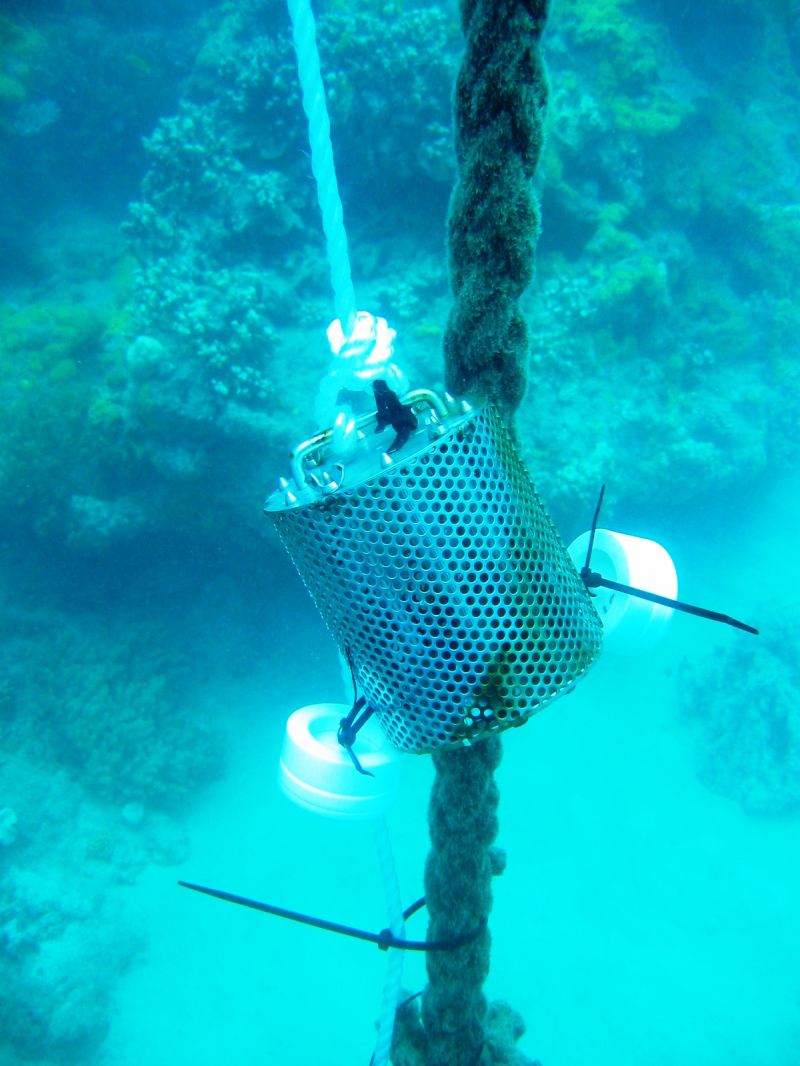
The aim of this component of the Reef Rescue Monitoring Program is to assess trends in the concentrations of specific herbicides and pesticides, primarily through routine monitoring at sites (Green Island, Low Isles, Fitzroy Island, Normanby Island, Dunk Island, Orpheus Island, Magnetic Island, Cape Cleveland, Pioneer Bay, Outer Whitsunday, Sarina Inlet, North Keppel Island) within 20km of the Queensland coast. The monitoring year for routine pesticide sampling is from May to April. The year is arbitrarily divided into “Dry Season” (May to October) and “Wet Season” (November– April) sampling periods for reporting purposes. Within each dry season, samplers are typically deployed for two months (maximum of three monitoring periods) and within each wet season, samplers are typically deployed for one month (maximum of six monitoring periods). The maximum number of samples which should be obtained from each location within each monitoring year is nine. Exposure to chemicals in the water is assessed with passive samplers. Passive samplers accumulate organic chemicals such as pesticides and herbicides from water until equilibrium is established between the concentration in water (CW ng.L-1) and the concentration in the sampler (CS ng.g-1). The concentration of the chemical in the water is estimated from calibration data obtained under controlled laboratory conditions (Booij et al., 2007). This calibration data consists of either sampling rates (RS L.day-1) for chemicals which are expected to be in the time-integrated sampling phase or sampler-water equilibrium partition coefficients (KSW L.g-1) for chemicals which are expected to be in the equilibrium sampling phase. Different types of organic chemicals need to be targeted using different passive sampling phases. The passive sampling techniques which are utilized in the MMP include: SDB-RPS Empore™ Disk (ED) based passive samplers for relatively hydrophilic organic chemicals with relatively low octanol-water partition coefficients (logKOW) such as the Photosystem II (PSII) herbicides (example: diuron). Polydimethylsiloxane (PDMS) and Semipermeable Membrane Devices (SPMDs) passive samplers for organic chemicals which are relatively more hydrophobic (higher log KOW) such as chlorpyrifos. The list of target chemicals was determined based on the following criteria: pesticides detected in recent studies, those recognised as a potential risk, analytical affordability, pesticides within the current analytical capabilities of Queensland Health Forensic and Scientific Services (QHFSS) and those likely to be accumulated within one of the passive sampling techniques (i.e. that exist as neutral species and are not too polar). Target Chemicals Bifenthrin, Fenvalerate (Pyrethroid, insecticides), Bromacilb , Tebuthiuron, Terbutrync, Flumeturon, Ametryn, Prometryn, Atrazine, Propazine, Simazine, Hexazinone, Diuron (PSII herbicides), Desethylatrazine, Desisopropylatrazine (PSII herbicide breakdown products (also active)), Oxadiazon Oxadiazolone (herbicide), Chlorfenvinphos , Chlorpyrifos, Diazinon, Fenamiphos, Prothiophos (Organophosphate insecticide), Chlordane, DDT, Dieldrin , Endosulphan, Heptachlor, Lindane (Organochlorine insecticides), Hexachlorobenzene (Organochlorine fungicide), Imidacloprid (Nicotinoid insecticide), Trifluralin (Dintiroaniline), Pendimethalin (Dinitroaniline herbicide), Propiconazole, Tebuconazole, (Conazole fungicides) Metolachlor (Chloracetanilide herbicide) Propoxur (Carbamate insecticide) PSII herbicides (ametryn, atrazine, diuron, hexazinone, flumeturon, prometryn, simazine and tebuthiuron and atrazine transformation products desethyl- and desiso-propyl – atrazine) sampled by the SDB-RPS ED samplers are also expressed as PSII herbicide equivalent concentrations (PSII-HEq) and are assessed against a PSII-HEq Index (Kennedy et al. 2010) for reporting purposes. PSII-HEq values were derived using relative potency factors (REP) collated from relevant laboratory studies for each chemical with respect to a reference PSII herbicide diuron (Jones and Kerswell, 2003; Mueller et al. 2008; Bengston-Nash et al 2005; Schmidt, 2005; Macova et al unpublished). If a given PSII herbicide is as potent as diuron, it will have a REP of 1. If it is more potent than diuron it will have a REP of >1, while if it is less potent than diuron it will have an REP of <1. Data Location: This dataset is saved in the eAtlas enduring data repository at: data\RRMMP\UQ_Mueller_Inshore-pesticides\GBR_RRMMP_UQ_Inshore-pesticides-2011