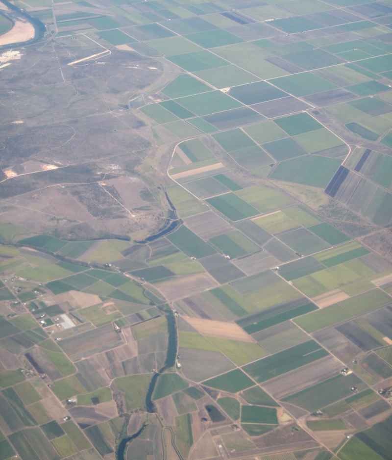
This dataset is a complete state-wide digital land use map of Queensland. The dataset is a product of the Queensland Land Use Mapping Program (QLUMP) and was produced by the Queensland Government. It presents the most current mapping of land use features for Queensland, including the land use mapping products from 1999, 2006 and 2009, in a single feature layer. This dataset was last updated July 2012. The dataset comprises an ESRI vector geodatabase at a nominal scale of 1:50,000 in coastal regions and 1:100 000 in Western Queensland. The layer is a polygon dataset with each class having attributes describing land use. Land use is classified according to the Australian Land Use and Management Classification (ALUMC) Version 7, May 2010. Five primary classes are identified in order of increasing levels of intervention or potential impact on the natural landscape. Water is included separately as a sixth primary class. Under the three-level hierarchical structure, the minimum attribution level for land use mapping in Queensland is secondary land use. Primary and secondary levels relate to land use (i.e. the principal use of the land in terms of the objectives of the land manager). The tertiary level includes data on commodities or vegetation, (e.g. crops such as cereals and oil seeds). Where required* and possible, attribution is performed to tertiary level. * QLUMP maps the land use classes of sugar and cotton to tertiary level. Each polygon has been attributed with "Year", denoting the time at which the mapping is current at. A map illustrating the currency of land use is available at www.derm.qld.gov.au/science/lump/background.html A representation is available for users to apply a symbology to the land use data, by secondary ALUMC. Some land uses that fall under the minimum mapping unit of 2 ha are not explicitly mapped but aggregated into the surrounding land use classess, for example cropping - sugar and grazing native vegetation, whereby tracks and farm infrastructure, road reserves and drainage lines are included.

This project seeks to ensure that planning for the future development of the Torres Strait Islands is sustainable and capable of taking into account ecological and social information, assets, risk and existing infrastructure. This Plan provides the following information for each island: •identification of key environmental assets; •identification of key land management issues; •identification of key infrastructure needs; •land use mapping identifying land suitable for development and conservation; and •land use for the future sustainable management. Methodology In 2007 the TSRA invited 15 of the Torres Strait Island community to participate in the Sustainable Land Use Study, funded by the NHT (now Caring for the Country). Based on submissions received, the communities of Boigu, Dauan, Erub, Iama, Masig and Saibai were accepted to be involved in the project as stage 1 pilot project. In 2009 the TSRA, via funding from the major infrastructure project, requested the Land Use Plans be extended to the remaining 9 communities of Hammond, Kubin, St. Pauls, Badu, Warraber, Poruma, Mabuyag, Ugar and Mer. Stage 1 occurred between 2007 and 2008. Stage 2 occurred between 2009 and 2010. Preliminary Consultation The project team met with all Community Council (prior to amalgamation) and Prescribed Bodies Corporate (PBC) to discuss the project objectives and methodology. Phase 1 - Fauna and Habitat Assessment. Field Study The project team undertook field studies on the islands to identify key environmental assets and associated land management issues, identify areas of conservation importance and undertake fauna identification. Phase 2 - Information Gathering & Research. The project team collated all available data for the islands to order to produce a compressive collection of information on the islands. Data included plans and surveys from major infrastructure projects, data collected as part of other TSRA projects (e.g. regional ecosystem mapping, tide levels) and well as existing State government data. Also during this phase, the project team undertook a literature review of natural resource management issues in the context of the Torres Strait. This research, along with local knowledge obtained by Community in Phase 5, provided the foundation for the best practice principles outlined in the Plan. Phase 3 - Constraints and Information Mapping. The project team produced a series of constraints and information mapping. This included: •analysis of the data collected in Phases 2&3; •analysis of existing spatial datasets, including aerial photographs, maps and satellite imagery; •analysis of Commonwealth and State legislation, policies, strategies, reports and community plans; •development and sourcing of relevant GIS data layers; •preparation of base mapping showing satellite imagery, slope analysis, coastal impacts and inundation, fauna and habitat values, bushfire risk, limited cultural heritage information, extent of service infrastructure.

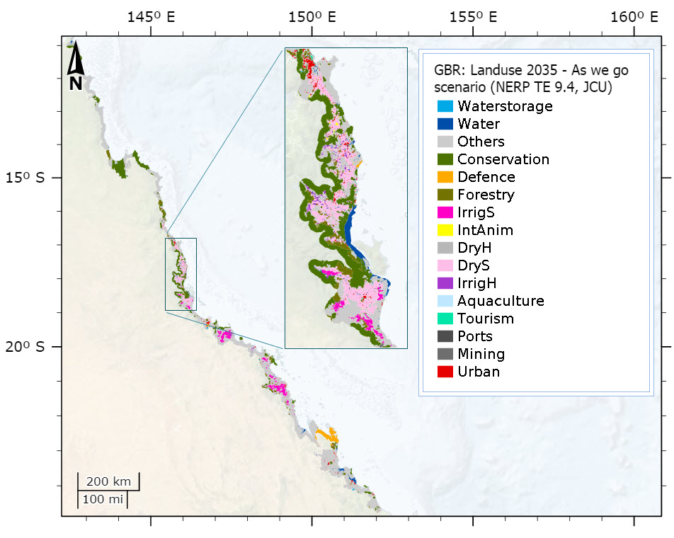
This dataset consists of different possible land use configurations along the Great Barrier Reef coastal zone for the future (year 2035) under eight different scenarios (plausible futures). Scenarios are not predictions and do not intend to show what the coastal zone will look like (this is impossible as the future of coastal development I highly uncertain, even on a short term basis, let alone 25 years). Instead, scenarios are used to depict some plausible futures under certain circumstances so that managers can understand the system better and the various ways the future might unfold. Scenarios are built to broaden the extremities of possibilities in order to assert the main differences. The scenarios are then used to conduct impact assessments and this helps managers better understand the connections between land spatial planning and the effects on the values of the GBR World Heritage Area. The results can also be incorporated in the process for spatial planning of coastal development. These scenarios were built using workshops and literature reviews and are based on different combinations of socio-economic factors driving the amount of change of the different land uses and of strength of governance systems (strong or weak). Figure 1 contains summaries of the storylines of the scenarios. These were translated in quantitative and spatial rules of change for land uses (transition matrix of land use change were created for each scenario and GIS layers were created for each spatial rule later combined to fit each scenario). The land use change modelling took several steps, all conducting the IDRISI Land Use Change Modeler. The first stage was to establish the best bio-physical predictors of change in land use. This was done using [see Bio-physical predictors of coastal Land use change between 1999 and 2009]. The outputs were transition probability maps for each change between one land use to another. The second stage was to use these transition probability maps, the quantitative matrices of change and the spatial rule layers to assign change and produce land use change configurations (the scenarios) to 2035. The modelling of the land use change was done at a 50m pixel scale. This was however aggregated to a resolution of 500m as presented here to ensure that the dataset is not seen as an accurate set of maps. The “predictive” power of change of the system is not expected to be accurate at the scale of 50m as the land use changes are applied in a probabilistic manner. As a result new allocated land may follow random pattern at the small scale and so the shape of the new areas do not necessarily have a structure that is natural for each land use type. An example of this is that in reality new residential developments tend to be rectangular in shape. However transitions to residential areas in the model tend to be scattered. To get around the excessive precision of the model this final dataset is aggregated to a resolution of 500m, where each pixel corresponds to the majority land use for that area. Format: The following rasters (GRID format) constitute the dataset of the spatially-explicit scenarios. They each represent land use maps for the terrestrial part of the Great Barrier Reef coastal zone in the past in 1999 (QLUMP data) and in 2009 (QLUMP data) and in the 8 scenarios produced as part of the NERP 9.4 project. See Figure 1 for detail of scenarios. 1999 : QLUMP 1999 data 2009 : QLUMP 2009 data AWG : Scenario As We Go (Business as usual in weak governance) EM : Scenario Export Management (Food and Minerals in strong governance) ER : Scenario Eco-Revolution (Green in strong governance) GW : Green Washing (Green in weak governance) RTC : Red Tape Cutting (Food and Minerals in weak governance) TH : Tourism Heaven (Tourism in strong governance) TOT : Twist on Trend (Business as Usual in strong governance) WFR : Way For Resorts (Tourism in weak governance) The classification of all rasters is as follow: PIXEL VALUE | PIXEL CLASS | NOTES 1 | Ocean | Not coastal zone 2 | Land | Not coastal zone 3 | Waterstorage | Human-made water storage (lakes/reservoirs) 4 | Water | Rivers, lakes estuaries etc 5 | Others | Mainly natural vegetation with grazing 6 | Conservation | Areas protected under IUCM status up to level IV 7 | Defence | Land with no entry permitted held by the Armies 8 | Forestry | Commercial plantations for timber 9 | IrrigS | Sugar cane fields requiring irrigation 10 | IntAnim | Indoor or improved pastures for high-density animal farms 11 | DryH | Crops, orchards, nut plantations, cotton with no irrigation 12 | DryS | Sugar cane fields with no irrigation 13 | IrrigH | Crops, orchards, nut plantations, cotton requiring irrigation 14 | Aquaculture | Land-based only 15 | Tourism | Areas built-up or used for tourism purposes 16 | Ports | Areas of commercial port infrastructure 17 | Mining | Areas under mining and related infrastructures 18 | Urban | Residential, retail and industrial areas (cities, towns) Part of the dataset includes a symbology layer filer that will automatically format the display in the best format for visualisation. classificationfromidrisi.lyr: This file contains the symbology (colour scheme for land use classes) to display the land maps and scenarios of the GBR coastal zone.

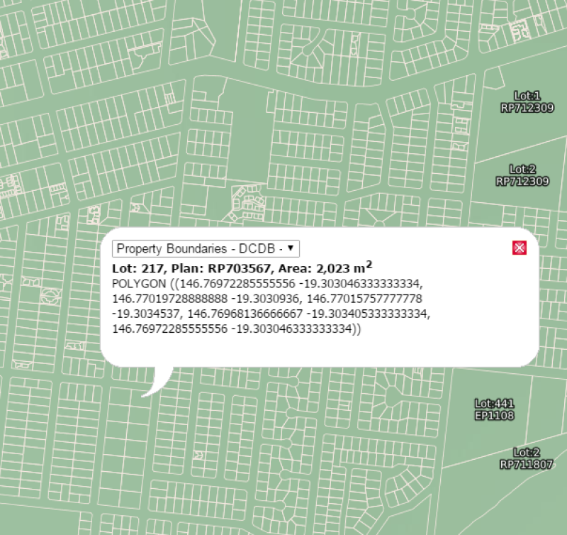
This polygon layer is a 'lite' version of the Digital Cadastral Database (DCDB) showing minimal attribute data about the property boundaries e.g.: base lot polygons, Lot and Plan attributes and an accuracy statement covering the whole of Queensland. See additional information also. This data is updated nightly on the QSpatial portal, but only infrequently on the eAtlas. The versions setup on the eAtlas are retained for historic purposes. This polygon layer is a 'lite' version of the base cadastre in the Digital Cadastral Database (DCDB) showing minimal attribute data about the property boundaries. The dataset does not contain information on volumetric, strata lots, multi level building format lots or secondary interest such as easements and covenants. A complete extract of the state or by an individual local government area is available from the Queensland Spatial Catalogue. EATLAS: This metadata record was created for the eAtlas and is not authoritative. It is based on a copy of the metadata supplied with the latest version of this dataset. Please contact QSpatial for the original metadata or more information. Data Dictionary 2023-05-29: LOT: Examples: 1, 36, 5026 PLAN: Examples: SP232048, RP195536, CA311276, PH251, EI835473 ACC_CODE: Examples: B&D ENTRY CONTROLLED - 0.1M, UPGRADE IMAGERY - 25M, UPGRADE ADJUSTMENT - 1M, STANDARD 1:2500 CADASTRAL MAP - 1.5M O_SHAPE_Le: Examples: 0.068803813631, 0.00093317039017. eAtlas Note: The units of this attributes is unknown, but it is not the shape perimeter in metres or km. O_SHAPE_Ar: Examples: 5.0887917895e-08 eAtlas Note: The units of this attributes is unknown, but it is not the shape area in square metres or square km. Change Log: - 2012-07-15: Original version setup in the eAtlas - 2016-08-18: The LOT_AREA attribute is no longer available. - 2023-05-29: Added a new version of the dataset.

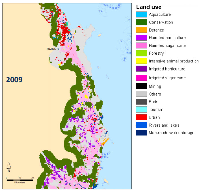
This dataset consist of inputs and intermediate results from the coastal scenario modelling. It is an analysis of the bio-physical factors that best explain the changes in QLUMP land use change between 1999 and 2009 along the Queensland coastal region for the classifications used in the future coastal modelling. Methods: The input layers (variables etc) were produced using a range of sources as shown in Table 1. Source datasets were edited to produce raster dataset at 50m resolution and reclassified to suit the needs for the analysis. The analysis was made using the IDRISI Land Use Change Modeler using multi-layer perceptron neural network with explanatory power of bio-physical variables. In this process a range of bio-physical layers such as slope, rainfall, distance to roads etc (see full list in Table 1) are used as potential explanatory variables for the changes in the land use. The neutral network is trained on a subset of the data then tested against the remaining data, thereby giving an estimate of the accuracy of the prediction. This analysis produces suitability maps for each of the transitions between different land use classifications, along with a ranking of the important bio-physical factors for explaining the changes. The 1999 - 2009 Land use change was analysed with of which 4 were found to be the strongest predictors of the change for various transitions between one land use and another. This dataset includes the rasters of the 4 best predictors along with a sample of the highest accuracy transition probability maps. Format: Table 1 (Table 1 NERP 9_4 e-atlas dataset) This table contains the list of names, short descriptions, data source and data manipulation for the input rasters for the land use change model All GIS files are in GDA 94 Albers Australia coordinate system. 1999.tif This layer shows a rasterised form of the QLUMP land use (clipped to the GBR coastal zone as defined in 9.4) for 1999 used for analysis of bio-physical predictors of land use change. The original QLUMP data was re-classified into 18 classes then rasterised at 50m resolution. This raster was then resampled to a 500m resolution. 2009.tif This layer shows a rasterised form of the QLUMP land use (clipped to the GBR coastal zone as defined in 9.4) for 2009 used for analysis of bio-physical predictors of land use change. The original QLUMP data was re-classified into 18 classes (with addition of tourism land use) then rasterised at 50m resolution. This raster was then resampled to a 500m resolution. Rainfall.rst This layer shows the average annual rainfall (in mm) sourced from the Average Yearly Rainfall Isohyets Queensland dataset (clipped to the GBR coastal zone as defined in 9.4) used for analysis of bio-physical predictors of land use change. The data was re-classified and resampled at 50m resolution. Slope.rst This layer shows the slope (in degrees) value at 50m pixel resolution (clipped to the GBR coastal zone as defined in 9.4) used for analysis of bio-physical predictors of land use change. The slope was derived from the Australian Digital Elevation Model in ArcGIS (using the Slope tool of the 3D analyst Tools) at a 200m resolution. The data was resampled at 50m resolution. SeaDist.rst This layer shows the distance (in m) to the nearest coastline (including estuaries) at 50m pixel resolution used for analysis of bio-physical predictors of land use change. It was created by applying an Euclidean distance function (in ArcGIS in the Spatial Analyst toolbox) to the “Mainland coastline” feature in the GBR features dataset available from GBRMPA. UrbanDist.rst This layer shows the distance (in m) to the nearest pixel of urban land use at 50m pixel resolution used for analysis of bio-physical predictors of land use change. It was created by applying an Euclidean distance function (in ArcGIS in the Spatial Analyst toolbox) to the QLUMP 2009 dataset on the selected urban polygons. Transition_potential_Other_to_DryHorticulture.rst This layer shows the probability for each pixel (50m resolution) of the coastal to transition from the land use class Other to Rain-fed Horticulture. Areas originally of a different land use class are given no values. This was produced by analysing the patterns of land use change between 1999 and 2009 in IRDISI as part of the Land Use Change Modeler where the main bio-physical variables affecting the pattern of change were identified. See details in the model results file. A high accuracy rate of 92% was calculated during testing. Land Change Modeler MLP Model Results_Rain-fed_horticulture.docx This shows the results of the analysis of change from land use Others to rain-fed horticulture between 1999 and 2009 using four variables: Distance to existing horticulture, Rainfall, Soil type and Slope. Transition_potential_Other_to_Drysugar.rst This layer shows the probability for each pixel (50m resolution) of the coastal to transition from the land use class Other to Rain-fed Sugar cane. Areas originally of a different land use class are given no values. This was produced by analysing the patterns of land use change between 1999 and 2009 in IRDISI as part of the Land Use Change Modeler where the main bio-physical variables affecting the pattern of change were identified. See details in the model results file. A high accuracy rate of 84% was calculated during testing. Land Change Modeler MLP Model Results_Rain-fed_sugar.docx This shows the results of the analysis of change from land use Others to rain-fed sugar between 1999 and 2009 using three variables: Rainfall, Soil type and Slope. Transition_potential_Other_to_Forestry.rst This layer shows the probability for each pixel (50m resolution) of the coastal to transition from the land use class Other to Forestry. Areas originally of a different land use class are given no values. This was produced by analysing the patterns of land use change between 1999 and 2009 in IRDISI as part of the Land Use Change Modeler where the main bio-physical variables affecting the pattern of change were identified. See details in the model results file. A good accuracy rate of 73% was calculated during testing. Land Change Modeler MLP Model Results_Forestry.docx This shows the results of the analysis of change from land use Others to Forestry between 1999 and 2009 using three variables: Rainfall, Soil type and Proximity to existing forestry. Transition_potential_Other_to_Urban.rst This layer shows the probability for each pixel (50m resolution) of the coastal to transition from the land use class Other to Urban. Areas originally of a different land use class are given no values. This was produced by analysing the patterns of land use change between 1999 and 2009 in IRDISI as part of the Land Use Change Modeler where the main bio-physical variables affecting the pattern of change were identified. See details in the model results file. A good accuracy rate of 75% was calculated during testing. Land Change Modeler MLP Model Results_Urban.docx This shows the results of the analysis of change from land use Others to Urban between 1999 and 2009 using two variables: Slope and Proximity to existing urban areas.

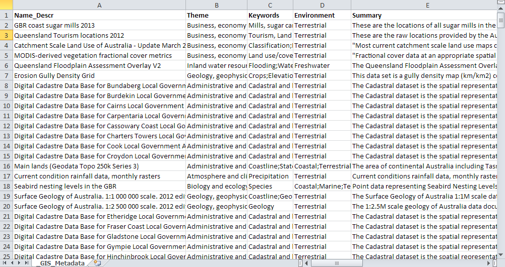
This dataset corresponds to a database of datasets that are relevant for the development of coastal development scenarios and impact assessments GBR. It corresponds to a list of all the datasets that were sourced as part of project 9.4. It contains basic information about each dataset along with the license that each dataset was obtained under and where the data can be sourced. This database is an excellent starting point for any others looking at obtaining data relevant for coastal management. Methods: Datasets were sourced from a large and various. They are presented in the database in their raw condition as downloaded or obtained. The database includes all metadata that was associated with them. The database is currently hosted on a server at the Centre of Excellence for Coral Reef Studies at James Cook University as is backed up weekly. Format: Coastal_zone_GIS_database.xlsx This is an excel file containing name and full description of all datasets. Each row corresponds to a different GIS file (either shapefile or raster). When dataset can be downloaded from a website with or without an open access licence, the link is included. For others, the best contact point is included.

This dataset corresponds to the polygon digitisation of tourism sites and sugar mills. The locations of the tourism sites were obtained from a commercial database of tourism operators (Australian Tourism Warehouse). The location of sugar mills was obtained from information gathered on the internet and point locations were created for each mill. These datasets were developed to fill in missing source datasets for the scenario modelling used for the coastal development modelling. The tourism dataset was incorporated to the 2009 QLUMP to provide inclusion of tourism land use in this dataset. The sugar mill dataset was developed to provide the distances from sugar land use to mill and determine the restrictions for future expansion. Methods: Tourism dataset: Tourism corresponds to the official definition used by the World Trade Organisation as "Tourism comprises the activities of persons travelling to and staying in places outside their usual environment for not more than one consecutive year for leisure, business and other purposes." It is generally accepted that in most instances tourism activities are conducted from approximately 50km of the domicile. The definition of tourism land use in this study is areas with infrastructure and areas of cleared land that would not have existed if it were not for demand from tourism and hospitality and the ability to gain economic benefits from that tourism as well as urban zones created to accommodate required staff and services, green areas etc. Tourism land use is not part of the QLUMP land use map. It was manually added to this dataset using data on tourism infrastructure from a private company (the Australian Tourism Data Warehouse) that registers tourism-related businesses and records geographical coordinates of businesses. Buffers around point locations were created to acknowledge for different sizes of buildings/carparks etc. Governmental data of recreational areas and airport facilities obtained from GeoScience Australia were added. The tourism layer was improved but is still not inclusive of all tourism area in 2013. Sugar mill dataset: The location of sugar mills was obtained from information gathered on the internet and point location were created for each mill. It includes Mossman mill, Pleystowe mill, Raceway mill, Marian mill, Farleigh mill, Tableland mill, Mulgrave central mill, Babinda mill, South Johnstone mill, Tully mill, Victoria mill, Macknade mill, Invicta mill, Pioneer mill, Kalamia mill, Inkerman mill, Prosperine mill, Plane creek mill. Format: GBR_TourismLandUse2013.shp (and associated files as part of shapeflie) This layer is a polygon shapefile representing all areas of land use associated with tourism in the GBR coastal zone. GBR_CoastSugarMills2013.shp (and associated files as part of shapeflie) This layer is a point shapefile containing all locations of sugar mills in operation as in March 2013 in the GBR coastal region or in close proximity.

The eAtlas delivers its mapping products via two Web Mapping Services, a legacy server (from 2008-2011) and a newer primary server (2011+) to which all new content is added. This record describes the primary WMS. This service delivers map layers associated with the eAtlas project (https://eatlas.org.au), which contains map layers of environmental research focusing on the Great Barrier Reef and its neighbouring coast, the Wet Tropics rainforests and Torres Strait. It also includes lots of reference datasets that provide context for the research data. These reference datasets are sourced mostly from state and federal agencies. In addition to this a number of reference basemaps and associated layers are developed as part of the eAtlas and these are made available through this service. This services also delivers map layers associated with the Torres Strait eAtlas. This web map service is predominantly set up and maintained for delivery of visualisations through the eAtlas mapping portal (https://maps.eatlas.org.au) and the Australian Ocean Data Network (AODN) portal (http://portal.aodn.org.au). Other portals are free to use this service with attribution, provided you inform us with an email so we can let you know of any changes to the service. This WMS is implemented using GeoServer version 2.13 software hosted on a Amazon Web Services (AWS) server. Associated with each WMS layer is a corresponding cached tiled service which is much faster then the WMS. Please use the cached version when possible. The layers that are available can be discovered by inspecting the GetCapabilities document generated by the GeoServer. This XML document lists all the layers, their descriptions and available rendering styles. Most WMS clients should be able to read this document allowing easy access to all the layers from this service. For ArcMap use the following steps to add this service: 1. "Add Data" then choose GIS Servers from the "Look in" drop down. 2. Click "Add WMS Server" then set the URL to "https://maps.eatlas.org.au/maps/wms?" Note: this service has over 1500 layers and so retrieving the capabilities documents can take a while. This services is operated by the Australian Institute of Marine Science and co-funded by the National Environmental Research Program Tropical Ecosystems hub.

The eAtlas delivers its mapping products via two Web Mapping Services, a legacy server (from 2008-2011) and a newer primary server (2011+) to which all new content it added. This record describes the legacy WMS. This service was decommissioned on in Jan 2024. This service delivered map layers associated with the eAtlas project (https://eatlas.org.au), and contained map layers of environmental research focusing on the Great Barrier Reef. The majority of the layers corresponding to Glenn De'ath's interpolated maps of the GBR developed under the MTSRF program (2008-2010). This web map service was predominantly maintained for the no decommissioned legacy eAtlas map viewer (https://maps.eatlas.org.au/geoserver/www/map.html). This WMS service was implemented using GeoServer version 1.7 software hosted on a server at the Australian Institute of Marine Science. Note: this service had around 460 layers of which approximately half the layers correspond to Standard Error maps, which were WRONG (please ignore all *Std_Error layers). This services was operated by the Australian Institute of Marine Science and co-funded by the MTSRF program. More details about this service is described on the eAtlas Legacy System webpage https://eatlas.org.au/content/legacy-mapping-system