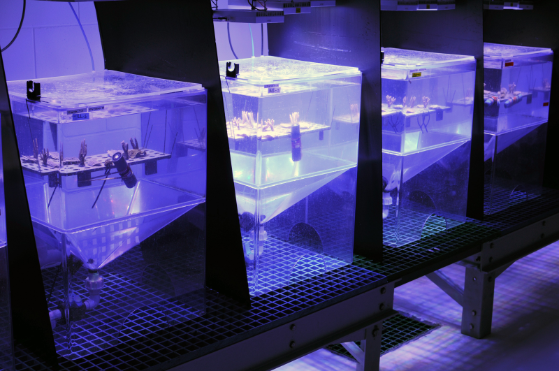
The dataset consists of four data files from a 20-day experiment to investigate different photophysiological responses of two species of coral (Acropora millepora and Pachyseris speciosa) to constant and variable daily light integrals. Methods: Eight partial colonies each of Pachyseris speciosa (from 5 – 8 m depth) and Acropora millepora (from 3 – 5 m depth) were collected from Davies Reef, central Great Barrier Reef, Australia (-18.823390, 147.6518563) in July 2016, and taken to the National Sea Simulator at the Australian Institute of Marine Science (AIMS), Townsville. Experiment consisted of four types of light exposure treatments, wherein nubbins from the partial colonies were either exposed to 20 days of high light (32 mol photons m-2 d-1), low light (6 mol photons m-2 d-1), or alternating variable light treatments. Four sets of photoacclimation and physiological responses were measured and the corresponding data has been placed in four separate csv files; (1) Fluorescence measurements were conducted using a diving pulse-amplitude modulated fluorometer (DPAM). Measurements were taken twice with the DPAM: once at 0.5 h before sunrise, to assess the maximum quantum yield of photosystem II (Fv/Fm), and at noon, after 0.5 h exposure to maximum irradiance, to assess effective quantum yield (PSII). For each nubbin, at least five measurements were taken from different regions on each nubbin and the values averaged. The excitation pressures on PSII, (see Ralph et al. 2016) was assessed to estimate the degree of photoinhibition versus light limitation. Non-photochemical quenching (NPQ), also derived from PAM pre-dawn and noontime measurements based on equations by Genty et al 1987, was measured to assess the amount of excess photon energy dissipated safely as heat. (2) At the end of the experiment, the concentration of chlorophyll a (photosynthetic) and total carotenoids (photosynthetic and photoprotective) of nubbins were compared between treatments. Tissue was removed from the skeleton with an air gun and filtered seawater, and homogenized. The slurry was centrifuged for 6-8 min at 1,500 g and the coral host supernatant was separated from the symbiont pellet. The pellet was then rinsed with filtered seawater and re-centrifuged at 10,000 g for 3 min prior to extraction. Pigments were obtained via a double extraction procedure (1 mL 95% ethanol at 4oC for 20 minutes each, with sonicator), and the absorbance was spectrophotomerically measured at 665, 664, 649 and 470 nm wavelengths. Concentrations of chlorophyll a and total carotenoids (µg/mL) were calculated based on equations by Lichtenthaler (1987) and Ritchie (2008) and standardized to nubbin surface area, which was estimated via a single wax dip protocol (Veal et al 2010). (3) At the end of the experiment, 18 nubbins were selected for respirometry measurements. Their ceramic plugs were carefully cleaned to remove algal growth. Nubbins were individually placed in 634 mL sealed stirred chambers that contained oxygen sensor spots (optodes), and the Firesting hardware/software (Pyroscience, Germany) was used to measure oxygen concentrations within the chambers every minute. Incubations ran for an hour each at ten light levels (0, 15, 40, 80, 120, 200, 300, 500, 700 and 1000 µmol photons m-2 s-1), measured with an upwards facing, calibrated, cosine corrected light sensor (meter LI-250A, sensor LI-192, Li-COR, USA). Water was flushed in the chambers at the beginning of each light level measurement. Rates of oxygen consumption (estimated respiration in the dark) and production (estimated net photosynthesis in the light) were standardized to coral surface area estimates derived from the wax dipping procedure. Photosynthesis to irradiance (P-I) curves were fitted to the data using a hyperbolic tangent fit, as described by Jassby and Platt (1976) using the ‘stats’ package (version 3.6.0) in the statistical platform R (version 3.4.0, R Development Core Team 2017). Parameters for maximum photosynthetic production (Pmax), saturation irradiance (Ik) and dark respiration (Rdark) for each treatment were estimated from fitted models. Net daily oxygen production (Pn) was calculated by predicting production using the P-I curves at actual logged experimental light levels, over a 24 h period. (4) Growth rates of A. millepora were assessed as differences in buoyant weight over time (Davies 1989). Nubbins were individually weighed to the nearest 0.001 g by suspending them on a tray below a semi-micro balance (Shimadzu AUW220D, Japan) in a water bath at ~25 OC. The percent change in buoyant weight between days 8 and 20 was assessed. Literature Cited Lichtenthaler HK. [34] Chlorophylls and carotenoids: Pigments of photosynthetic biomembranes. Methods in Enzymology. 148: Academic Press; 1987. p. 350-82. Ritchie RJ. Universal chlorophyll equations for estimating chlorophylls a, b, c, and d and total chlorophylls in natural assemblages of photosynthetic organisms using acetone, methanol, or ethanol solvents. Photosynthetica. 2008;46(1):115–26. Veal CJ, Holmes G, Nunez M, Hoegh-Guldberg O, Osborn J. A comparative study of methods for surface area and three-dimensional shape measurement of coral skeletons. Limnology and Oceanography: Methods. 2010;8(5):241-53. doi: 10.4319/lom.2010.8.241. Jassby AD, Platt T. Mathematical formulation of the relationship between photosynthesis and light for phytoplankton. Limnology and Oceanography. 1976;21(4):540-7. doi: 10.4319/lo.1976.21.4.0540. Davies S. Short-term growth measurements of corals using an accurate buoyant weighing technique. Marine Biology. 1989;101(3):389–95. doi: 10.1007/BF00428135. Ralph PJ, Hill R, Doblin MA, Davy SK (2016) Theory and application of pulse amplitude modulated chlorophyll fluorometry in coral health assessment. In: Diseases of Coral, pp. 506–523. Format: The dataset consists of four separate components, stored as .csv files, pertaining to the different physiological aspects used to understand coral responses to variable light conditions; fluorometry (85KB), pigment analysis (6KB), respirometry (9KB) and growth (1KB). Data Dictionary: pam.csv - Date: Date of sampling (DD/MM/YY) - Group: Which sampling group the individual was placed in. - Treatment: Which treatment the individual was in, where HL is High Light, LL is Low Light, VLH is Variable Light starting High and VLL is Variable Light starting Low. - Tank: Tank number each nubbin resided in - Species: Either Acropora millepora or Pachyseris speciosa - Coral_ID: Colony identification - Fo_mean: minimum fluorescence yield in dark - Fm_mean: maximum fluorescence yield in dark - DA_yield; Refers to the maximum quantum yield, quantifies the maximum potential for photosynethesis through proportion of available photosystems in a dark-adapted state (dimensionless) - F_mean; steady-state fluorescence yield in light - Fm._mean; maximum fluorescence yield in light - LA_yield: refers to the effective quantum yield, quantifying the relative number of open to closed photosystems in a light-adapted state (dimensionless) - Qm; Excitation pressure of photosystem II, which is a relationship between effective and maximum quantum yields and gives an idea of the relative light-limitation or photoinhibitory stress on the coral (dimensionless) pigments.csv - Treatment: Which treatment the individual was in, where HL is High Light, LL is Low Light, VLH is Variable Light starting High and VLL is Variable Light starting Low. - Tank: Tank number - Species: Either Acropora millepora or Pachyseris speciosa - Coral_ID: Colony identification - Individual_ID: Individual identification - Surface: Relevant for P. speciosa only, refers to whether tissue was taken from the top or the bottom of the nubbin - surfaceArea: Surface area in cm2 - ChlA: estimated total of chlorophyll a (micrograms) per individual coral nubbin - Caro: estimated total of total carotenoids (micrograms) per individual coral nubbin - chlaSA: estimate of chlorophyll a by surface area (micrograms per cm2) per individual coral nubbin - caroSA: estimate of total carotenoids by surface area (micrograms per cm2) per individual coral nubbin - Ratio: Ratio of chlorophyll a to carotenoids respirometry.csv - Date: Date of sampling (DD/MM/YY) - Group: Which sampling group the individual was placed in, based solely on order of respirometry run - Pattern: Whether the treatment was constant (HL or LL) or variable (VLH or VLL) - Treatment: Which treatment the individual was in, where HL is High Light, LL is Low Light, VLH is Variable Light starting High and VLL is Variable Light starting Low - Light: Whether light levels were low or high - Irradiance (umolEm-2s-1); Instantaneous irradiance measurement in micromoles photons per m2 per second - Species: Either Acropora millepora or Pachyseris speciosa - ID: Individual ID - Production_mgO2hr-1: Oxygen production based on respirometry in milligrams of oxygen produced per hour weight.csv (only Acropora millepora in this dataset) - Treatment: Which treatment the individual was in, where HL is High Light, LL is Low Light, VLH is Variable Light starting High and VLL is Variable Light starting Low - Tank: Tank number - Coral_ID: Colony and individual ID - Percent_change: percent change in buoyant weight Data Location: This dataset is filed in the eAtlas enduring data repository at: data\2016-18-NESP-TWQ-2\2.3.1_Benthic-light\AU_NESP-TWQ-2.3.1_AIMS_BenthicLight_experiment2

This dataset is a complete state-wide digital land use map of Queensland. The dataset is a product of the Queensland Land Use Mapping Program (QLUMP) and was produced by the Queensland Government. It presents the most current mapping of land use features for Queensland, including the land use mapping products from 1999, 2006 and 2009, in a single feature layer. This dataset was last updated July 2012. The dataset comprises an ESRI vector geodatabase at a nominal scale of 1:50,000 in coastal regions and 1:100 000 in Western Queensland. The layer is a polygon dataset with each class having attributes describing land use. Land use is classified according to the Australian Land Use and Management Classification (ALUMC) Version 7, May 2010. Five primary classes are identified in order of increasing levels of intervention or potential impact on the natural landscape. Water is included separately as a sixth primary class. Under the three-level hierarchical structure, the minimum attribution level for land use mapping in Queensland is secondary land use. Primary and secondary levels relate to land use (i.e. the principal use of the land in terms of the objectives of the land manager). The tertiary level includes data on commodities or vegetation, (e.g. crops such as cereals and oil seeds). Where required* and possible, attribution is performed to tertiary level. * QLUMP maps the land use classes of sugar and cotton to tertiary level. Each polygon has been attributed with "Year", denoting the time at which the mapping is current at. A map illustrating the currency of land use is available at www.derm.qld.gov.au/science/lump/background.html A representation is available for users to apply a symbology to the land use data, by secondary ALUMC. Some land uses that fall under the minimum mapping unit of 2 ha are not explicitly mapped but aggregated into the surrounding land use classess, for example cropping - sugar and grazing native vegetation, whereby tracks and farm infrastructure, road reserves and drainage lines are included.

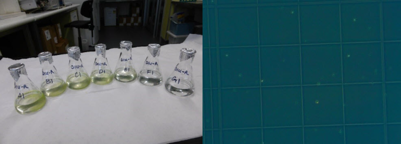
This dataset shows the effects of herbicides (detected in the Great Barrier Reef catchments) on the growth rates (from cell density data) and photosynthesis (effective quantum yield) on the green algae Raphidocelis subcapitata during laboratory experiments conducted during 2019. The aims of this project were to develop and apply standard ecotoxicology protocols to determine the effects of Photosystem II (PSII) and alternative herbicides on the growth and photosynthetic efficiency of the green algae Raphidocelis subcapitata. Growth bioassays were performed over 3-day exposures using herbicides that have been detected in the Great Barrier Reef catchment area (O’Brien et al. 2016). Effects of herbicides on the photophysiology of Raphidocelis subcapitata, measured by chlorophyll fluorescence as the effective quantum yield (Delta F/Fm') were investigated using pulse amplitude modulation (PAM) fluorometry after 72 h herbicide exposure. These toxicity data will enable improved assessment of the risks posed by PSII and alternative herbicides to microalgae for both regulatory purposes and for comparison with other taxa. Methods: The chlorophyte Raphidocelis subcapitata (strain CS-327) was purchased from the Australian National Algae Supply Service, Hobart (CSIRO). Cultures of R. subcapitata were established in MLA medium (Bolch and Blackburn 1996). Cultures were maintained in sterile 250 mL Erlenmeyer flasks as batch cultures in exponential growth phase with weekly transfers of 1 - 3 mL of a 7 day-old R. subcapitata suspension to 100 mL MLA medium under sterile conditions. Clean culture solutions were maintained at 26 ± 2°C, and under a 12:12 h light:dark cycle (91 ± 12 µmol photons m–2 s–1). Herbicide stock solutions were prepared using PESTANAL (Sigma-Aldrich) analytical grade products (HPLC greater than or equal to 98%): diuron (CAS 330-54-1), haloxyfop-p-methyl (CAS 72619-32-0) and imazapic (CAS 104098-48-8). The selection of herbicides was based on application rates and detection in coastal waters of the GBR (Grant et al. 2017, O’Brien et al. 2016). Stock solutions were prepared in sterile 100 - 500 mL glass volumetric flasks using milli-Q water. Diuron and haloxyfop-p-methyl were dissolved using analytical grade acetone (final concentration < 0.01% (v/v) in exposures). Imazapic was dissolved in methanol (final concentration less than or equal to 0.01% (v/v) in exposure). Cultures of R. subcapitata were exposed to a range of herbicide concentrations over a period of 72 h. Inoculum was taken from cultures in exponential growth phase (4 – 7 day-old cultures). A R. subcapitata working suspension was prepared in a 100 mL volumetric flask. A 1:10 and 1:100 dilutions were prepared and counted using a haemocytometer under a compound microscope to determine appropriate dilution volumes. The pre-determined inoculum was added to 50 mL of each test and control treatment replicates to the required dilution (3 – 3.1 x 104 cells/ mL). In each toxicity test, a control (no herbicide) and solvent control (if used) treatments were added to support the validity of the test protocols and to monitor continued performance of the assays. All treatment concentrations were prepared in 0.5x strength MLA medium. Replicates were incubated at 26.6 ± 0.5 °C under a 12:12 h light:dark cycle (190 ± 14 µmol photons m–2 s–1). Sub-samples were taken from each replicate to measure cell densities of algal populations at 72 h using a haemocytometer and photographed under phase contrast conditions. Cell counts were done either manually or using ImageJ from microscope photographs (Rueden et al 2017). Specific growth rates (SGR) were expressed as the logarithmic increase in cell density from day i (ti) to day j (tj) as per equation (1), where SGRi-j is the specific growth rate from time i to j; Xj is the cell density at day j and Xi is the cell density at day i (OECD 2011). SGR i-j = [(ln Xj - ln Xi )/(tj - ti )] (day-1) (1) SGR relative to the control treatment was used to derive chronic effect values for growth inhibition. A test was considered valid if the SGR of control replicates was greater than or equal to 0.92 day-1 (OECD 2011). Physical and chemical characteristics of each treatment were measured at 0 h and 72 h including pH, electrical conductivity and temperature. Chamber temperature was also logged in 15-min intervals over the total test duration. Analytical samples were taken at 0 h and 72 h. Effects of herbicides on the photophysiology of R. subcapitata, measured by chlorophyll fluorescence as the effective quantum yield (Delta F/Fm'), were investigated at 72 h using a mini-PAM fluorometer (mini-PAM, Walz, Germany). Light adapted minimum fluorescence (F) and maximum fluorescence (Fm') were determined and effective quantum yield was calculated for each treatment as per equation (2)(Schreiber et al. 2002). Delta F/Fm’ = (Fm’-F)/Fm’ (2) Mini- PAM settings were set to ETR-F = 0.84, F-Offset = 92, measuring light frequency = 3, measuring intensity = 4, gain = 3; damp = 3. Saturation pulse settings: intensity = 6, width = 0.6. Mean percent inhibition in SGR and Delta F/Fm' of each treatment relative to the control treatment was calculated as per equation (3)(OECD 2011), where Xcontrol is the average SGR or Delta F/Fm' of control and Xtreatment is the average SGR or Delta F/Fm' of single treatments. % Inhibition = [(X control - X treatment )/X control] x 100 (3) Format: Raphidocelis subcapitata herbicide toxicity data_eAtlas.xlsx Data Dictionary: There are two tabs for diuron in the spreadsheet. The first tab corresponds to the specific growth rate (SGR) data; the second tab is the pulse amplitude modulation (PAM) fluorometry data. For haloxyfop and imazapic there is one tab, corresponding to specific growth rate (SGR) data. The last tab of the dataset shows the measured water quality (WQ) parameters (pH, electrical conductivity and temperature) of each herbicide test. Diu – Diuron Halo – Haloxyfop Imaz – Imazapic For each ‘herbicide’_SGR tab: SGR = specific growth rate – the logarithmic increase from day 0 to day 3 Nominal (µg/L) = nominal herbicide concentrations used in the bioassays; SC denotes solvent control which is no herbicide and contains less than 0.01% v/v solvent carrier as per the treatments Measured (µg/L) = measured concentrations analysed by The University of Queensland Rep = Replicate: for SGR, notation is 1-3; for PAM data, notation is 1-3 T3_CellsPer_ml = cell density at day 3 ln(day3) = natural logarithm of cell density at day 3 Average T0_CellsPer_ml = average cell density at day 0 ln(Day0) = natural logarithm of cell density at day 0 For Diuron_PAM tab: PAM = pulse amplitude modulation fluorometry to calculate effective quantum yield (light adapted) Nominal (µg/L) = nominal herbicide concentrations used in the bioassays; SC denotes solvent control which is no herbicide and contains less than 0.01% v/v solvent carrier as per the treatments Measured (µg/L) = measured concentrations analysed by The University of Queensland Rep = Replicate: for SGR, notation is 1-3; for PAM data, notation is 1-3 Delta F/Fm' = effective quantum (light adapted) yield measured by a Pulse Amplitude Modulation (PAM) fluorometer References: Bolch, C. J. S. and Blackburn S. I. (1996). Isolation and purification of Australian isolates of the toxic cyanobacterium Microcystis aeruginosa Kütz. Journal of Applied Phycology 8, 5-13 Grant, S., Gallen, C., Thompson, K., Paxman, C., Tracey, D. and Mueller, J. (2017) Marine Monitoring Program: Annual Report for inshore pesticide monitoring 2015-2016. Report for the Great Barrier Reef Marine Park Authority, Great Barrier Reef Marine Park Authority, Townsville, Australia. 128 pp, http://dspace-prod.gbrmpa.gov.au/jspui/handle/11017/13325 O’Brien, D., Lewis, S., Davis, A., Gallen, C., Smith, R., Turner, R., Warne, M., Turner, S., Caswell, S. and Mueller, J.F. (2016) Spatial and temporal variability in pesticide exposure downstream of a heavily irrigated cropping area: application of different monitoring techniques. Journal of Agricultural and Food Chemistry 64(20), 3975-3989. OECD (2011) OECD guidelines for the testing of chemicals: freshwater alga and cyanobacteria, growth inhibition test, Test No. 201. https://search.oecd.org/env/test-no-201-alga-growth-inhibition-test-9789264069923-en.htm (accessed 28 August 2019). Rueden, C.T., Schindelin, J., Hiner, M.C. et al. (2017) ImageJ2: ImageJ for the next generation of scientific image data. BMC Bioinformatics 18:529, PMID 29187165, doi:10.1186/s12859-017-1934-z Data Location: This dataset is filed in the eAtlas enduring data repository at: data\nesp3\3.1.5_Pesticide-guidelines-GBR

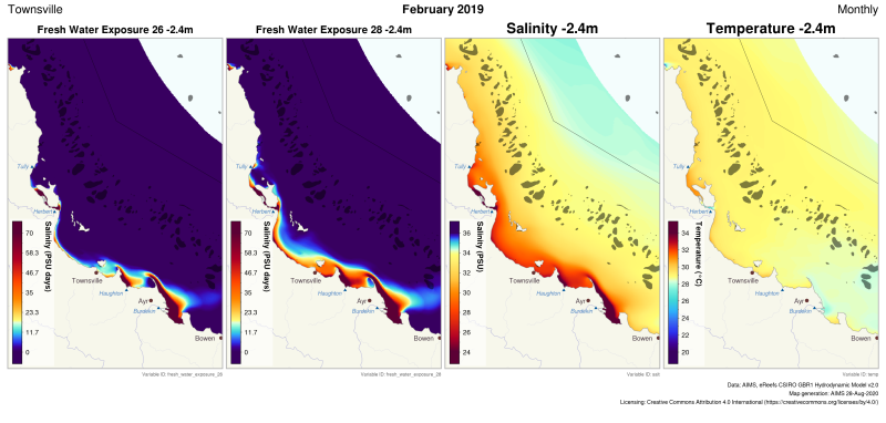
This generated data set contains exposure products derived from the eReefs CSIRO hydrodynamic model v2.0 (https://research.csiro.au/ereefs) outputs at both 1km and 4km resolution, generated by the AIMS eReefs Platform (https://ereefs.aims.gov.au/ereefs-aims). These exposure products are derived from the original hourly model outputs available via the National Computing Infrastructure (NCI) (https://dapds00.nci.org.au/thredds/catalogs/fx3/catalog.html), and have been re-gridded from the original curvilinear grid used by the eReefs model into a regular grid so that the data files can be easily loaded into standard GIS software. These products are made available via a THREDDS server (https://thredds.ereefs.aims.gov.au/thredds/) in NetCDF format. For more information about the eReefs hydrodynamic modelling see https://research.csiro.au/ereefs/models/models-about/models-hydrodynamics/. This dataset contains the following exposure products: * FRESH WATER EXPOSURE The freshwater exposure products calculate the level of exposure to salinity levels below a threshold over a calendar month. The standard thresholds used in the freshwater exposure products generated by the AIMS eReefs Platform are 26 and 28 PSU (refer to the attributes attached to the variables in the NetCDF files to confirm). These were chosen as different species have different tolerances to freshwater exposure, and the most appropriate level is not currently known. Method: The freshwater exposure is calculated from the sum of the daily average salinity below the exposure threshold. Salinity levels above the threshold don't contribute at all to the exposure. Salinity levels below the threshold contribute in proportion to the amount below the threshold. As a result with a threshold of 28 PSU and an exposure to 22 PSU for 3 days the freshwater exposure would be (28-22)*3 = 18 PSU days. The same exposure at 25 PSU would take 6 days (28-25)*6 = 18 PSU days. This method of calculating exposure is conceptually very similar to temperature exposure measured in Degree Heating Weeks, where the higher the temperature is above the typical maximum summer temperature the faster the heat stress occurs. For freshwater exposure the stress occurs when the salinity drops below the threshold value. The lower the salinity the faster the exposure accumulates. More research is needed to determine if this is the best method for estimating stress from freshwater. A more detailed description of the processing, especially exposure calculations and regridding, is available in the "Technical Guide to Derived Products from CSIRO eReefs Models" document (https://nextcloud.eatlas.org.au/apps/sharealias/a/aims-ereefs-platform-technical-guide-to-derived-products-from-csiro-ereefs-models-pdf ). Data Dictionary: The variables found in the freshwater exposure products document the threshold used to calculate that variable. For example: - fresh_water_exposure_29p5 : threshold = 29.5 - fresh_water_exposure_28 : threshold = 28.0 - fresh_water_exposure_26 : threshold = 26.0 Depths: Depths at 1km resolution: -2.35m Depths are 4km resolution: -1.5m Limitations: This dataset is based on a spatial and temporal model and as such is an estimate of the environmental conditions. It is not based on in-water measurements, and thus will have a spatially varying level of error in the modelled values. It is important to consider if the model results are fit for the intended purpose.

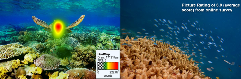
This dataset resulted from two inter-linked research streams. The first stream was related to the application of eye-tracking technology and an online survey in studying natural beauty. The second stream is related to the development of an Artificial Intelligence (AI)-based system recognising and assessing the beauty of natural scenes. Due to differences in data collection and data analysis, details of research methods used for each research stream are described in three separated data records. This record that describes the common elements and goals of the three parts to the research. Within these research streams, three datasets were developed. These include: Eye tracking - containing the outcome documents of eye-tracking experiment conducted within the project framework Online survey - includes a survey format document and three subfolders showing how each section of the survey was designed and outcome of each section (i.e. conjoint analysis, picture rating and open question) Algorithm data reflecting how a computer-based system for automated assessment of image attractiveness is developed Format and methods: The project dataset has multiple parts containing data of different formats and methods. Details of each dataset are discussed in the corresponding data records. Data Dictionary: See data dictionaries in the following data report forms: Becken, S., Connolly R., Stantic B., Scott N., Mandal R., Le D., (2018), Eye-tracking data report form, Griffith Institute for Tourism Research Report No 15. Becken, S., Connolly R., Stantic B., Scott N., Mandal R., Le D., (2018), Online survey data report form, Griffith Institute for Tourism Research Report No 15. Becken, S., Connolly R., Stantic B., Scott N., Mandal R., Le D., (2018), Algorithm data report form, Griffith Institute for Tourism Research Report No 15. References: Further information can be found in the following publication: Becken, S., Connolly R., Stantic B., Scott N., Mandal R., Le D., (2018), Monitoring aesthetic value of the Great Barrier Reef by using innovative technologies and artificial intelligence, Griffith Institute for Tourism Research Report No 15. Becken, S., Connolly R., Stantic B., Scott N., Mandal R., Le D., (2018), Eye-tracking data report form, Griffith Institute for Tourism Research Report No 15. Becken, S., Connolly R., Stantic B., Scott N., Mandal R., Le D., (2018), Online survey data report form, Griffith Institute for Tourism Research Report No 15. Becken, S., Connolly R., Stantic B., Scott N., Mandal R., Le D., (2018), Algorithm data report form, Griffith Institute for Tourism Research Report No 15. Data Location: This dataset is filed in the eAtlas enduring data repository at: data\nesp3\3.2.3_Aesthetic-Values-GBR

This generated data set contains summaries (daily, monthly) of the eReefs CSIRO river tracers model v2.0 (https://research.csiro.au/ereefs) outputs at 4km resolution, generated by the AIMS eReefs Platform (https://ereefs.aims.gov.au/ereefs-aims). These summaries are derived from the original daily model outputs available via the National Computing Infrastructure (NCI) (https://dapds00.nci.org.au/thredds/catalogs/fx3/catalog.html), and have been re-gridded from the original curvilinear grid used by the eReefs model into a regular grid so that the data files can be easily loaded into standard GIS software. These summaries are updated in near-real time daily and are made available via a THREDDS server (https://thredds.ereefs.aims.gov.au/thredds/ ) in NetCDF format. In addition to the variables containing single river data, we have added an 'all_rivers' variable which shows the total river water concentration (%) by combining all river output into a single variable. The eReefs river tracers model output contains passive river tracer results derived from version 2.0 of the 4km-resolution regional-scale hydrodynamic model of the Great Barrier Reef (GBR4). In the model, tracers are released at the river's mouth into its surface flow. These tracers move with the ocean currents, becoming more dilute as they spread out and mix with the ocean water, allowing the concentration of river water to be tracked over time. These tracers show the fraction of the water, at any given location, associated with each river. This model configuration and associated results dataset may be referred to as "GBR4_H2p0_Rivers" according to the eReefs simulation naming protocol. Description of the data: The data shows the percentage concentration of river water in the marine water. This is a good proxy for the extent of flood plumes associated with the major rivers along the Queensland coastline flowing into the Great Barrier Reef Marine Park. Flood plumes deliver sediments and nutrients into the ocean, both of which can result in detrimental effects on seagrass and reef habitats. Very low salinity concentrations in flood plumes can also cause bleaching and mortality on inshore reefs (this occurred during the flooding on Virago shoal off Townsville after the 2019 floods).This dataset represents only the concentration of river water in the marine environment. It does not model the changes in salinity, the nutrients levels or the sediment concentration in the water. These variables are calculated in the eReefs hydrodynamic model (salinity) and the biogeochemical model (nutrients and sediment). The river tracer is uniquely useful for tracing the origin of flood water back to the source river. The movement of the river water is driven by the surface ocean currents, that are driven largely by the wind. During most months the south easterly trade winds push the plumes back toward the coast in a northern direction. During the monsoon season, which is strongest between February and March, the winds drop and become more variable in direction. This means that flooding during these months is more variable in direction, occasionally moving southward and out to sea, sometimes reaching the mid shelf reefs. The width of the continental shelf narrows north of Townsville, resulting in it being easier for the flood plumes to reach the mid and outer reefs. Most significant flood plumes occur during the wet season from November to April. Flood plumes are less likely during the dry season from May to October. The plumes from some of the larger rivers can travel extensive distances during large flooding events. For example during 2019, flood waters from the Burdekin river travelled 700 km north along the coast, reaching Lizard Island. In 2017 the flood waters of the Fitzroy river reached the Whitsundays (450 km north) and the Normanby river water reached the tip of Cape York (440 km north). The rivers with the biggest discharge resulting in large flood plumes the Burdekin, Herbert, Tully, Johnstone, Russel, Mulgrave, Normanby, Fitzroy and Mary rivers. The following is a summary of the rivers with significant flood plumes during each year: 2015 Normanby, Mulgrave (minor), Johnstone (minor), Herbert (minor), Fitzroy, Mary 2016 Normanby, Mulgrave (minor), Tully (minor), Burdekin, Fitzroy, Mary (minor) 2017 Normanby, Johnstone, Herbert (minor), Tully (minor), Burdekin (major), Pioneer, Fitzroy (major), Burnett (minor), Mary (minor) 2018 Normanby, Mulgrave, Johnstone, Tully, Herbert, Burdekin, Mary (minor) 2019 Normanby, Daintree, Mulgrave, Johnstone, Tully, Herbert, Haugton (major), Burdekin (major), Pioneer (minor) 2020 Normanby (minor), Burdekin (minor), Fitzroy (minor) 2021 Normanby, Mulgrave (minor), Johnstone (minor), Tully (minor), Herbert, Burdekin (major), Fitzroy, Burnett (minor), Mary (minor) 2022 Normanby (minor), Daintree (minor), Mulgrave (minor), Johnstone (minor), Burdekin, Burnett (minor), Mary (major), Brisbane (minor), Logan (minor) 2023 Normanby, Herbert, Haugton (minor), Burdekin, Fitzroy (minor) Method: A description of the processing, especially aggregation and regridding, is available in the "Technical Guide to Derived Products from CSIRO eReefs Models" document (https://nextcloud.eatlas.org.au/apps/sharealias/a/aims-ereefs-platform-technical-guide-to-derived-products-from-csiro-ereefs-models-pdf). Data Dictionary: Variables: - nom: [% river water] Normanby - mul: [% river water] Mulgrave and Russell - jon: [% river water] Johnstone - her: [% river water] Herbert - bur: [% river water] Burdekin - fit: [% river water] Fitzroy - mar: [% river water] Mary - dai: [% river water] Daintree - bar: [% river water] Barron - tul: [% river water] Tully - hau: [% river water] Haughton - don: [% river water] Don - con: [% river water] O'Connell - pio: [% river water] Pioneer - bnt: [% river water] Burnett - fly: [% river water] Fly - cal: [% river water] Calliope - boy: [% river water] Boyne - cab: [% river water] Caboolture - log: [% river water] Logan - pin: [% river water] Pine - bri: [% river water] Brisbane - all_rivers: [% river water] Aggregation of all river outputs. This is a numerically addition of all single river variables to determine the total river water concentration (%). - time: [days since 1990-01-01 00:00:00 +10] Time - zc: [m] Z coordinate (depth) - depth slices - latitude: [degrees_north] Latitude (geographic projection) - longitude: [degrees_east] Longitude (geographic projection) Dimensions: - time - k (variable: zc) - latitude - longitude Depths: This data set contains the following depths, which are a subset of the depths available in the source data set [m]: -0.5, -1.5, -3.0, -5.55, -8.8, -12.75, -17.75, -23.75, -31.0, -39.5, -49.0, -60.0, -73.0, -88.0, -103.0, -120.0, -145.0. Limitations: This dataset is based on a spatial and temporal model and as such is an estimate of the environmental conditions. It is not based on in-water measurements. Furthermore, it should be noted that the river tracer product tracks the concentration of river water. It does not track sediment or nutrient in the water. As part of research into determining a suitable river concentration threshold for visualisations, we undertook many comparisons between the estimated flood plume extent from eReefs and those visible in Sentinel 2 satellite imagery. From this we found that the plume extent from eReefs was generally accurate to within about 10 km, with the most likely reason for the difference being slight errors in the model due to wind. The strength and direction of the wind is the predominant factor in determining the spread of the flood plumes. As a result any small errors in the modelling of the wind will lead to errors in the flood plume boundaries. The eReefs hydrodynamic model is driven by wind data from the Bureau of Meteorology's Access-R weather model, which is a forecast. It has a resolution of 12 km and so it is surprising that the eReefs model is as spatially accurate as it is. Part of the reason for this is that while the wind occasionally pushes the plumes offshore, the main determinant of the distribution is the dynamics of buoyant plumes. The rotation of the Earth acts to deflect to the left (in the Southern Hemisphere) any relative increase in motion between fluid layers. One such relative motion is a buoyant plume flowing over the top of denser ocean water. Deflected left on a river discharging along an east coast means it being pushed towards the coast. Thus, the plumes are trapped near the coast. The distance to which they spread from the coast is also set by this balance between density driven flow and the Earth’s rotation, something ocean models are very good at. The eReefs model tracks the percentage river water concentrations to very low levels, such as 1 part per million. At very low concentrations there is likely to not be ecologically relevant. When comparing the plume extents from the river tracer data with flood plumes visible in Sentinel 2 imagery we found that a concentration of 1% river water closely aligned with the visible edge of the flood plumes, where the water is darker and slightly green due to the increased levels of algae in the water.

This dataset contains the code for the Android application “COTS Control Centre Decision Support Tool” (CCC-DST). The CCC-DST is one part of the “COTS Control Centre Decision Support System” (CCC-DSS) which is a hardware and software solution, comprising 32 Samsung Galaxy Tab Active2 tablets. The tablets run a kiosk operating system and provide three data collection apps, developed for GBRMPA by ThinkSpatial, and three decision support components developed by CSIRO as part of the NESP COTS IPM Research Program. The CCC-DST application is an implementation of the principles outlined in “An ecologically-based operational strategy for COTS Control” (Fletcher, et al., 2020). Methods: The COTS Control Centre Decision Support Tool (CCC-DST) is part of the COTS Control Centre Decision Support System (CCC-DSS). The CCC-DSS is a combined hardware and software solution developed by CSIRO as part of the National Environmental Science Program (NESP) Integrated Pest Management (IPM) Crown-of-thorns starfish (COTS) Research Program to help guide on-water decision making and implement the ecologically-informed management program outlined in the report “An ecologically-based operational strategy for COTS Control: Integrated decision making from the site to the regional scale” (Fletcher, Bonin, & Westcott, 2020). The COTS Control Centre DSS is built around a fleet of 32 ruggedised Samsung Galaxy Tab Active2 Android tablets, along with a suite of three data collection apps, developed for the Great Barrier Reef Marine Park Authority (GBRMPA) by ThinkSpatial, and three decision support components developed by CSIRO as part of the NESP COTS IPM Research Program. The fleet of tablets are able to be managed remotely, including locating hardware and updating software, using the Samsung Knox Manage Enterprise Mobility Management platform, and run a custom kiosk launcher. Data is shared between the apps that make up the CCC-DSS within a tablet using the Android file system, between tablets on a vessel independent of cellular connectivity with the Android Nearby Communications protocol, and with GBRMPA’s Eye on the Reef Database when cellular networking is available. In addition to designing and implementing the overarching CCC-DSS system, CSIRO has developed a suite of three software components, consisting of the main Decision Support Tool (CCC-DST), a Data Explorer functionality, which is currently implemented as part of the CCC-DST but may, in future, be separated into a second app, and a utility Data Sync Tool for sharing data between tablets when internet connectivity is not available. Details of the underlying philosophy and implementation notes of the CCC-DST can be found in the technical report: Fletcher C. S. and Westcott D. A. (2021) The COTS Control Centre: Supporting ecologically-informed decision making when and where the decisions need to be made. Report to the National Environmental Science Program. Reef and Rainforest Research Centre Limited, Cairns (189pp.). Architecture: In general, Android applications are designed to require minimal memory footprint by cycling data out of their sqlite database on the fly as required. This is an efficient method of designing lightweight apps coexisting on mobile hardware will limited memory and processing capacity. It works well for some of the tasks required of the NESP COTS Control Centre apps, but is not intuitively suited to all the functionality required. This is especially the case for situations where data must be compared longitudinally through time or across many Sites or Reefs in order to guide decision making. On the other hand, because the COTS Control Centre is run on dedicated hardware of known specification and containing only the suite of apps necessary to guide on-water actions, we can bias the design of our system towards functionality within the hardware being used, rather than optimising for universal efficiency. As a result, the COTS Control Centre apps were developed with a hybrid philosophy that aims to target the data loaded into memory to that required to inform a decision, and which structures the data in memory using custom classes that reflect the actual data being analysed. This approach puts an emphasis on both logical database design and well-structured custom types to support the functionality of the apps, each of which are described in further detail in the sections that follow. The apps were developed in stages, starting with prototypes early in 2016. As a result, they retain some legacy functionality, such as the use of loaders rather than the ViewModel and Room functionality introduced in Android after this time. They also include components, such as a ContentProvider framework, that were expected to be important at one stage in app development, but which are not deeply leveraged in the current configuration. The structure of the apps also reflects the fact that their development will continue to incorporate feedback from on-water operators, as well as scientific advances in biological understanding, field measurements, and management strategies. As a result, in some places a more general programming approach has been favoured over more optimised code in order to maintain or provide flexibility to incorporate new functionality in future. Note: The database file has been omitted from the source files. The details of the database layout can be found in the technical report (section 2.2): Fletcher C. S. and Westcott D. A. (2021) The COTS Control Centre: Supporting ecologically-informed decision making when and where the decisions need to be made. Report to the National Environmental Science Program. Reef and Rainforest Research Centre Limited, Cairns (189pp.) Format: Java application (Android) References: Fletcher C. S. and Westcott D. A. (2021) The COTS Control Centre: Supporting ecologically-informed decision making when and where the decisions need to be made. Report to the National Environmental Science Program. Reef and Rainforest Research Centre Limited, Cairns (189pp.) Fletcher C. S., Bonin M. C, Westcott D. A.. (2020) An ecologically-based operational strategy for COTS Control: Integrated decision making from the site to the regional scale. Reef and Rainforest Research Centre Limited, Cairns (65pp.). Data Location: This dataset is filed in the eAtlas enduring data repository at: data\custodian\2019-2022-NESP-TWQ-5\5.1_COTS-pest-management

This dataset consists of three data files (spreadsheets) from a two month aquarium experiment manipulating pCO2 and light, and measuring the physiological response (photosynthesis, growth, protein and pigment content) of the adult and juvenile stages of two species of tropical corals (Acropora tenuis and A. hyacinthus). Methods: We conducted a two-month, 24-tank experiment at AIMS’s SeaSim facility, in which recently settled juvenile- and adult-colonies of the corals Acropora tenuis and A. hyacinthus were exposed to four light treatments (high, medium, low and variable intensities), fully crossed with two levels of dissolved CO2 (400 and 900 ppm). The four light treatments used in the experiment (low, medium, high and variable) each had 12 hrs of light and a five hour ramp, but at different intensities. The high light treatment had a noon max of 500 µmol photon m-2 s-1 and a DLI of 12.6 mol photon m-2, the medium treatment had a noon max of 300 µmol photon m-2 s-1 and a DLI of 7.56 mol photon m-2, while the low light treatment had a noon max of 100 µmol photon m-2 s-1 and a DLI of 2.52 mol photon m-2. The variable treatment oscillated on a five day cycle, with four days at the low treatment intensity, a ramp day at the medium, then four days at the high treatment intensity. The mean DLI of the variable treatment was therefore the same as medium treatment. Light intensities were checked in each individual aquaria with a calibrated underwater light sensor (Licor, USA). The variable light treatment allowed us to investigate how these corals acclimate to a changing light environment, and to see if responses are due to limitation under low light, or inhibition under high light (i.e. coral responses in the variable treatment would resemble the low or high light treatments), or whether light has a cumulative effect regardless of variability (i.e. coral responses in the variable treatment would resemble the medium light treatment). Adult corals were collected from Davies Reef (18.30 S, 147.23 E) while juveniles were spawned from adults at AIMS’s SeaSim facility. After two months of experiment exposure, growth (change in corallite number) and survivorship were assessed in the juvenile corals from photographs, while growth (buoyant weight changes), and protein and pigment content were assessed in the adults after tissue stripping following standard procedures. Briefly, each adult coral nubbin was water-picked in 10 mL of ultra-filtered seawater (0.04 µm) to remove coral tissue. This tissue slurry was then homogenised and centrifuged to separate coral and symbiont components following. Total coral protein content was quantified from the coral tissue supernatant with the DC protein assay kit (Bio-Rad Laboratories, Australia), while Symbiodinium pigments in the pellet were determined spectrophotometrically (Lichtenthaler 1987, Richie 2008). Protein content was standardised to nubbin surface area, estimated with the single wax-dipping technique (Veal et al. 2010), while pigment content was standardised by nubbin surface area, as well as by protein content. A series of photophysiological measurements for the effective (PhiPSII) and maximum (Fv/Fm) quantum yield of photosystem II were made on the adults with a pulse amplitude modulated fluorometer over the final ten days of the experiment. Photosynthetic pressure (Qm: 1 - PhiPSII / Fv/Fm) and relative electron transport rate (rETR: PhiPSII * PAR) were calculated (Ralph et al. 2016) to see how they were responding to their light environment. References: Lichtenthaler HK (1987) Chlorophylls and carotenoids: Pigments of photosynthetic biomembranes. Methods in Enzymology, 148, 350–382. Ralph PJ, Hill R, Doblin MA, Davy SK (2016) Theory and application of pulse amplitude modulated chlorophyll fluorometry in coral health assessment. In: Diseases of Coral, pp. 506–523. Ritchie RJ (2008) Universal chlorophyll equations for estimating chlorophylls a, b, c, and d and total chlorophylls in natural assemblages of photosynthetic organisms using acetone, methanol, or ethanol solvents. Photosynthetica, 46, 115–126. Veal CJ, Carmi M, Fine M, Hoegh-Guldberg O (2010) Increasing the accuracy of surface area estimation using single wax dipping of coral fragments. Coral Reefs, 29, 893–897.

This dataset shows the effects of herbicides (detected in the Great Barrier Reef catchments) on growth rates (from surface area and biomass) and photosynthesis (effective quantum yield) on the aquatic fern Azolla pinnata during laboratory experiments conducted in 2019. The aims of this project were to develop and apply standard ecotoxicology protocols to determine the effects of Photosystem II (PSII) and alternative herbicides on the growth and photosynthetic efficiency of the aquatic fern Azolla pinnata. Growth bioassays were performed over 14-day exposures using herbicides that have been detected in the Great Barrier Reef catchment area (O’Brien et al. 2016). Chronic effects of herbicides on the photophysiology of A. pinnata, measured by chlorophyll fluorescence as the effective quantum yield (Delta F/Fm’) were investigated using PAM fluorometry after 14-day herbicide exposure. These toxicity data will enable improved assessment of the risks posed by PSII and alternative herbicides to aquatic macrophytes for both regulatory purposes and for comparison with other taxa. Methods: The aquatic fern Azolla pinnata was sourced from Watergarden Paradise Nursery, NSW. Cultures were established in IRRI2 medium (Pereira & Carrapiço 2009). Cultures were maintained in 10 L tubs containing 3–5 L IRRI2 as batch cultures with weekly transfers to fresh medium. Clean culture solutions were maintained at 26 ± 1 °C, under a 12:12 hr light:dark cycle (65-77µmol photons m–2 s–1). Herbicide stock solutions were prepared using PESTANAL (Sigma-Aldrich) analytical grade products (HPLC greater than or equal to 98%): diuron (CAS 330-54-1), fluometuron (CAS 2164-17-2), fluroxypyr (CAS 69377-81-7), haloxyfop-p-methyl (CAS 72619-32-0), imazapic (CAS 104098-48-8), isoxaflutole (CAS 141112-29-0) and triclopyr (CAS 5535-06-3). The selection of herbicides was based on application rates and detection in coastal waters of the GBR (Grant et al. 2017, O’Brien et al. 2016). Stock solutions were prepared in 100 mL glass volumetric flasks using milli-Q water. Diuron, haloxyfop-p-methyl and isoxaflutole were dissolved using analytical grade acetone (< 0.01% (v/v) in exposures). Imazapic was dissolved in methanol (less than 0.01% (v/v) in exposure). No solvent carrier was used for the preparation of the remaining herbicide stock solutions. Cultures of A. pinnata were exposed to a range of herbicide concentrations over a period of 14 days. Fronds were selected from actively growing cultures free of overt disease or deformity. Four triplicate fronds each comprising eight ramets were added to 100 mL of each herbicide solution concentration and control treatment. In each toxicity test, control (no herbicide) and solvent control (if used) treatments were added to support the validity of the test protocols and to monitor continued performance of the assays. Experiments were conducted in IRRI2 medium (Pereira & Carrapiço 2009) with solutions replaced at Day 7. Three replicates of each treatment solution and control were prepared and incubated at 26.6 ± 0.5 °C under a 12:12 h light:dark cycle (90 ± 6 µmol photons m–2 s–1). Each replicate treatment was photographed at a standard height to estimate surface area at Day 0 and Day 14. Biomass of a representative numbers of fronds were weighed to 4 significant figures using an analytical balance after blotting for 15 seconds to remove excess moisture. Fronds from each treatment replicate were weighed at Day 14 using the same technique. Specific growth rates (SGR) were expressed as the logarithmic increase in surface area or biomass from day i (ti) to day j (tj) as per equation (1), where SGRi-j is the specific growth rate from time i to j; Xj is the surface area or biomass at day j and Xi is the surface area or biomass at day i (OECD 2006). SGR i-j = [(ln Xj - ln Xi )/(tj - ti )] (day-1) SGR relative to the control / solvent control treatment was used to derive chronic effect values for growth inhibition. A test was considered valid, if the SGR for frond number or surface area of control replicates was greater than or equal to 0.0.0495 day-1 (OECD 2014). Physical and chemical characteristics of each treatment were measured at 0, 7 and 14 days on new and old treatment solutions for pH, electrical conductivity and temperature. Temperature was also logged in 15-min intervals over the total test duration. Analytical samples were taken at 0 and 14 days. Chronic effects of herbicides on the photophysiology of A. pinnata, measured by chlorophyll fluorescence as the effective quantum yield (Delta F/Fm’), were investigated at 14 days using PAM fluorometry (mini-PAM, Walz, Germany). Light adapted minimum fluorescence (F) and maximum fluorescence (Fm') were determined and effective quantum yield was calculated for each treatment as per equation (2)(Schreiber et al. 2002). Delta F/Fm’ = (Fm’-F)/Fm’ Mini- PAM settings were set to ETR-F = 0.84, F-Offset = 46, measuring light frequency = 3, measuring intensity = 4, gain = 2; damp = 3. Saturation pulse settings: intensity = 6, width = 0.6. Mean percent inhibition in SGR and Delta F/Fm’ of each treatment relative to the control treatment was calculated as per equation (3)(OECD 2006), where Xcontrol is the average SGR or Delta F/Fm’ of control and Xtreatment is the average SGR or Delta F/Fm’ of single treatments. % Inhibition = [(X control - X treatment )/X control] x 100 Format: Azolla pinnata herbicide toxicity data_eAtlas.xlsx Data Dictionary: There are two or three tabs for each herbicide in the spreadsheet. The first tab corresponds to the specific growth rate – surface area (SGR-SA) data; the second tab is biomass (SGR-B) data; and the pulse amplitude modulation (PAM) fluorometry data. The last tab of the dataset shows the measured water quality (WQ) parameters (pH, electrical conductivity and temperature) of each herbicide test. Where value equals '-', measurement not taken. Diu – Diuron Fluo - Fluometuron Flur - Fluroxypyr Halo – Haloxyfop Imaz - Imazapic Isox - Isoxaflutole Tri – Triclopyr For each ‘herbicide’_SGR tab: SGR = specific growth rate - the logarithmic increase from day 0 to day 14 as either surface area (SA) (mm2) or biomass (B) (g) Nominal (µg/L) = nominal herbicide concentrations used in the bioassays; SC denotes solvent control which is no herbicide and contains less than 0.01% v/v solvent carrier as per the treatments Measured (µg/L) = measured concentrations analysed by The University of Queensland Rep = replicate notation is 1-3 T14_Growth = surface area (mm2) or biomass (g) at day 14 ln(day14) = natural logarithm of surface area (mm2) or biomass (g) at day 14 Average T0_Growth = surface area (mm2) or biomass (g) at day 0 ln(day0) = natural logarithm of surface area (mm2) or biomass (g) at day 0 For each ‘herbicide’_PAM tab: PAM = pulse amplitude modulation fluorometry to calculate effective quantum yield (light adapted) Nominal (µg/L) = nominal herbicide concentrations used in the bioassays; SC denotes solvent control which is no herbicide and contains less than 0.01% v/v solvent carrier as per the treatments; Measured (µg/L) = measured concentrations analysed by The University of Queensland notation is 1-3; for PAM data, notation is 1-3 Delta F/Fm' = effective quantum (light adapted) yield measured by a Pulse Amplitude Modulation (PAM) fluorometer References: Grant, S., Gallen, C., Thompson, K., Paxman, C., Tracey, D. and Mueller, J. (2017) Marine Monitoring Program: Annual Report for inshore pesticide monitoring 2015-2016. Report for the Great Barrier Reef Marine Park Authority, Great Barrier Reef Marine Park Authority, Townsville, Australia. 128 pp, http://dspace-prod.gbrmpa.gov.au/jspui/handle/11017/13325 O’Brien, D., Lewis, S., Davis, A., Gallen, C., Smith, R., Turner, R., Warne, M., Turner, S., Caswell, S. and Mueller, J.F. (2016) Spatial and temporal variability in pesticide exposure downstream of a heavily irrigated cropping area: application of different monitoring techniques. Journal of Agricultural and Food Chemistry 64(20), 3975-3989. OECD (2006) Current approaches in the statistical analysis of ecotoxicity data. OECD Publishing. OECD (2014) Test No. 238: Sediment-Free Myriophyllum Spicatum Toxicity Test, OECD Guidelines for the Testing of Chemicals, Section 2, OECD Publishing, Paris. Pereira, A.L., and Carrapiço, F. (2009) Culture of Azolla filiculoides in artificial conditions. Plant Biosystems, 143(3), 431-434 Rueden, C.T., Schindelin, J., Hiner, M.C. et al. (2017) ImageJ2: ImageJ for the next generation of scientific image data. BMC Bioinformatics 18:529, PMID 29187165, doi:10.1186/s12859-017-1934-z Data Location: This dataset is filed in the eAtlas enduring data repository at: data\nesp3\3.1.5_Pesticide-guidelines-GBR

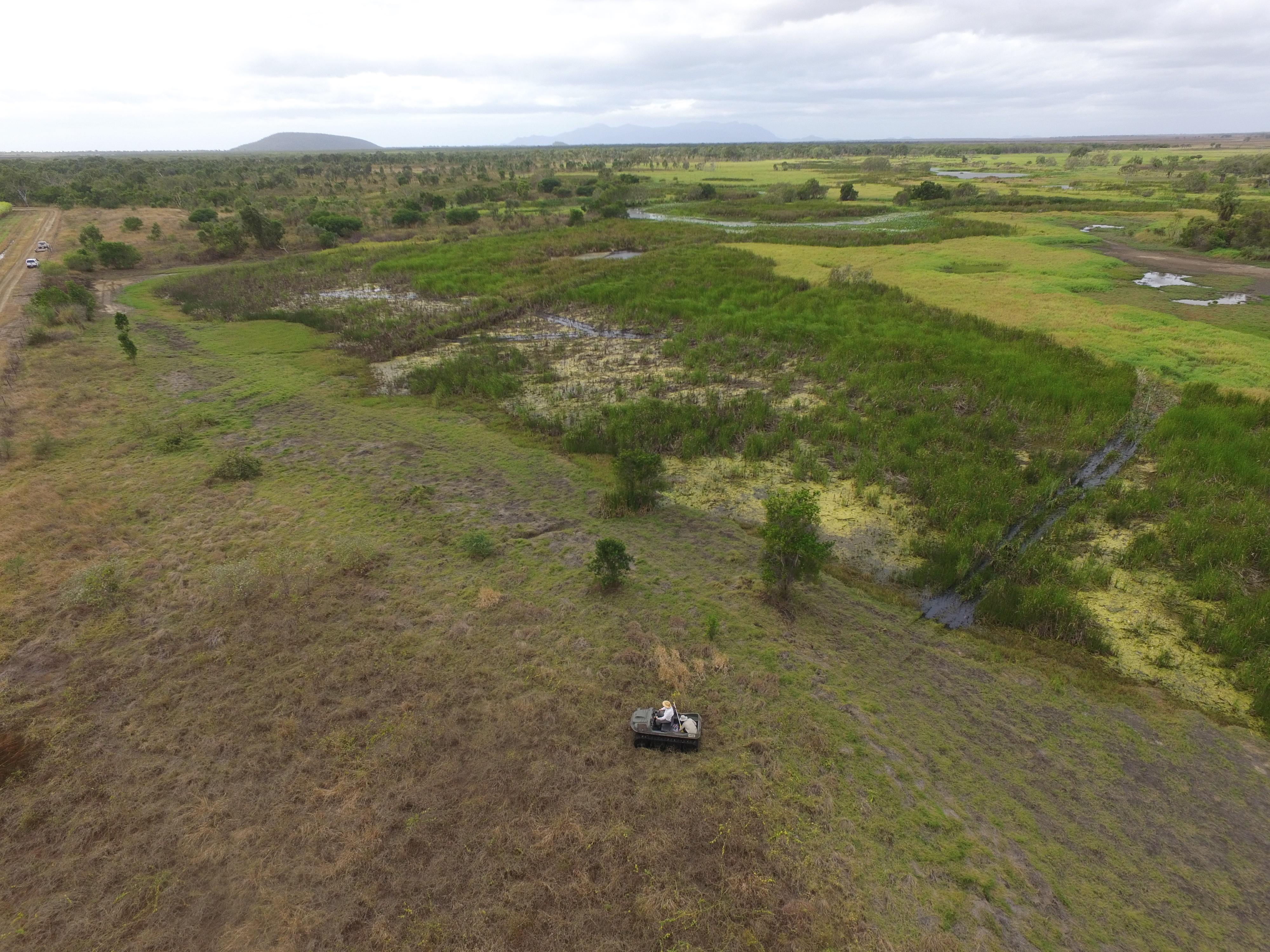
This data set contains high frequency logging data to measure water depth, water temperature and electrical conductivity in project wetland sites. Coastal wetlands adjacent to the Great Barrier Reef (GBR) have incredible environmental, cultural and economic value. Despite this, many floodplains in the GBR catchments have been modified, impacted or lost entirely because of continuing land use change (such as agricultural, aquaculture, peri-urban/urban, and industrial expansion). Of the floodplains and their wetlands remaining many now provide severely reduced aquatic and avian habitat, due to alien weed infestation and poor water quality. A large number of coastal wetlands have also lost their connectivity with estuaries that flow into the GBR lagoon (e.g. due to earth bunding), which can impact marine and freshwater aquatic (diadromous) species that have a critical estuary lifecycle phase, and rely on this connectivity between the reef and shallow tidal and freshwater wetlands. The overall project objective is to evaluate existing and future coastal wetland system repair investments, covering a combination of project sites across Great Barrier Reef catchment area, to explicitly evaluate how these projects achieve biodiversity improvements, water quality benefits and connectivity with downstream marine coastal habitats. Methods: High frequency water depth logging Water depth, temperature and electrical conductivity were monitored by loggers (CTD-Diver, Eijkelkamp Soil & Water, Netherlands) located in the wetland. The loggers captured data from the bottom of the water column (~ 10 cm above the soil surface) every 20 minutes, and were downloaded as part of routine maintenance visits. Each logger was installed inside a PVC pipe (3m height, 90mm diameter) that was attached to a steel star picket. Loggers were attached to a stainless steel wire cord that was attached to the top of the PVC pipe for easy retrieval (downloading the data and maintenance). The loggers were downloaded every few months. For more details see: Canning, A., Adame F., Waltham, N. J., (2020) Evaluating the services provided by ponded pasture wetlands in Great Barrier Reef catchments – Tedlands case study. Report to the National Environmental Science Program. Reef and Rainforest Research Centre Limited, Cairns (23pp.). Waltham, N. J. & Canning, A. (2020) Exploring the potential of watercourse repair on an agricultural floodplain. Report to the National Environmental Science Program. Reef and Rainforest Research Centre Limited, Cairns (75pp.). Format: All data are in Excel format. References: Canning, A., Adame F., Waltham, N. J., (2020) Evaluating the services provided by ponded pasture wetlands in Great Barrier Reef catchments – Tedlands case study. Report to the National Environmental Science Program. Reef and Rainforest Research Centre Limited, Cairns (23pp.). Waltham, N. J. & Canning, A. (2020) Exploring the potential of watercourse repair on an agricultural floodplain. Report to the National Environmental Science Program. Reef and Rainforest Research Centre Limited, Cairns (75pp.). Data Location: This dataset is filed in the eAtlas enduring data repository at: data\custodian\2019-2022-NESP-TWQ-5\5.13_Coastal-wetland-systems-repair