About pygmy blue whales
Blue whales are the largest animals in the world. The pygmy blue whale (Figure 1) is a sub-species which is only a few metres shorter (~24 m) than the largest in the group; the Antarctic blue whale (~30 m). The species is listed on the International Union for Conservation of Nature (IUCN) as Data Deficient, and under the Australian Environment Protection and Biodiversity Conservation (EPBC) Act as Endangered (read about these categories). Although these are very large species, their population numbers are low and they spend most of their life under water and using waters far from shore (off the continental shelf) and so they are difficult to study.
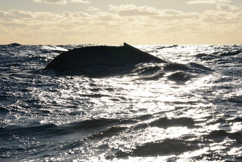
Figure 1. A pygmy blue whale in deep water off North West Cape, Western Australia during the northern migration.
They are found in the Southern, Indian and South Pacific Ocean (see world ocean map). The group of pygmy blue whales which visits western & southern Australia is known as the Eastern Indian Ocean Pygmy Blue. They migrate along the WA coastline from summer feeding grounds in the Perth Canyon, Bonney upwelling and Sub-tropical Convergence zone to Indonesia in winter where scientists think they breed. This migratory path with potential feeding stop-overs may conflict with coastal and offshore activities for hydrocarbon and mineral resource (e.g. iron ore shipping) exploitation on the north-western coast and shelf area of Australia. Impact assessment and mitigation of these activities and other pressures in the region are difficult without accurate data on whale movement behaviour and where they spend time for different activities such as for feeding.
To assist in recovery of the population, spatial areas of importance to pygmy blue whales, known as Biologically Important Areas (BIA), have been identified by the Australian Government. These are areas where aggregations of individuals display biologically important behaviour such as calving, foraging, resting or migration. However, the BIAs in the north-west were established with little spatial data and relied in great part on expert input and therefore have some uncertainty associated with them. Due to this they are classified as “Possible foraging” areas, with one off the coast of Ningaloo and another near Scott Reef.
Here, the AIMS team and collaborators Centre for Whale Research and Curtin University set out to address this uncertainty in the important foraging areas for this species and their migration pathways and distribution to better assess overlap with anthropogenic activities and ensure effective management of potential threats to this population. We did this by deploying satellite tags at NW Cape during their northward migration and also made use of the pre-existing satellite tag deployments on pygmy blue whales from the more southern areas. We also used data from existing noise loggers (underwater hydrophones mounted on the sea floor to listen for and record whale songs) provided by Industry and new deployments of noise loggers. We used the combined data to model and map the spatial distribution of pygmy blue whales and define areas of importance for these whales off Western Australia with a focus on the north-west where data are limited and where many anthropogenic threats occur.
Tracking pygmy blue whales to identify important areas
AIMS deployed six satellite linked GPS tags on pygmy blue whales at Northwest Cape, Western Australia between May-June 2019-2020, and four satellite linked GPS tags and two pop-off archival tags at Perth Canyon in April 2021 (Figure 2). In addition, we compiled data from 10 previously deployed pygmy blue whale satellite tags; nine tagged at Perth Canyon, between March-April 2009 and 2011 and one tagged in the Bonney Upwelling region of South Australia in March 2015 during their outward migration to Indonesia. We used this data to calculate how much time whales spent in each location and identify important areas for feeding, breeding and migration. For each of these activities, we identified key areas used by most of the whales most of the time.
Figure 2. The AIMS and CWR team attempting to get close enough to a pygmy blue whale to attach a satellite tag.
Movement behaviour of the whales occurred mostly at the continental shelf edge and slope and was predominantly fast and directed with short (a few days) periods of slow movement and ‘milling’, indicative of foraging, in between. Pygmy blue whales had high use (both in time and number of whales) along the Ningaloo Coast up to the Rowley Shoals from April to June on their northern migration to the Banda and Molucca Seas in Indonesia.
Our analysis showed a good overlap between the important foraging areas we calculated in the southern part of Western Australia and the Known Foraging BIA off Perth Canyon (Figure 3). However, minimal overlap existed between the important foraging areas we calculated in the north-west and the Possible Foraging BIAs off Ningaloo and Scott Reef (Figure 3). This suggests that Possible Foraging BIA boundaries may need to be reviewed. In addition, the high use of this broad area by pygmy blue whales, the existence of foraging movement behaviour and our (and others) observations of feeding whales suggests that the ‘possible’ classification for the Ningaloo BIA should also be reviewed.
Figure 3. Map showing the core areas for occupancy (purple), core areas for number of overlapping whales (blue), the grid cells where foraging/breeding movement behaviour present (orange), and the overlap between these three metrics of pygmy blue whale spatial use (red) representing the most important foraging/breeding areas. Green polygons represent the Known and Possible Foraging BIAs delineated by the Australian Government. Grey line represents the extent of the shelf.
The most important migration areas we calculated from these tagged whales is encompassed by the Migration BIA (Figure 4) which is good news. However, the entire area where migration behaviour occurred (shown in brown on Figure 4) indicates that the migratory pathway of pygmy blue whales is much wider than the Migration BIA. Our tracking data also showed that the tracked whales did not use the shelf area (indicated by the grey line in Figure 3), suggesting the Distribution BIA could be overestimating the area used by whales.
Figure 4. Map showing the core areas for number of overlapping whales (blue), the grid cells where migratory movement behaviour was present (brown), and the overlap between these two metrics of pygmy blue whale spatial use representing the most important areas used during migration (red). Pink polygons represent the migration BIA delineated by the Australian Government and the purple polygon represents the distribution (the entire area of use) BIA in Australia. Grey line represents the extent of the shelf.
Using the presence of pygmy blue whales calls recorded on noise loggers, we also showed higher density of singing whales in the southern extent of the north-west of WA during their northern and southern migrations (Figure 5 and Figure 6). However, unlike the tracking data, the data suggest some minor use of the NW Shelf mostly in the deeper parts of the shelf along the Ningaloo Coast and towards Barrow Island and off Dampier.
Figure 5. Predicted number of singing whales (singers/km2∙day) for May (northern migration) each month from the top ranked Random Forrest model.
Figure 6. Predicted number of singing whales (singers/km2∙day) for November (southern migration) each month from the top ranked Random Forrest model.
Conclusion
By analysing pygmy blue whale tracking data and their songs recorded on noise loggers across the Northwest, we have been able to identify the times of the year and the areas that are most important to them for foraging and migration. This information is important for assessing threats to pygmy blue whales and for revising the current extent of the BIA boundaries off Western Australia.
Animation of blue whale tracks obtained from the satellite tags
The animation shows the blue whale tagged at off WA during their northern migration to their breeding grounds in the Banda Sea. Some of the longest tracks also show the whales migrating back south.
Detailed explanation
Analysis of pygmy blue whale satellite tracking data
We applied a state space model to the raw tracking data from the satellite tags that provides an index of behaviour (called move persistence, g) with each location, where slower swimming with high turn angles is characteristic of resident behaviours such as foraging or breeding, and faster and more direct movements characterise migration. To identify spatial distribution (the entire area that whales use) and areas of highest use, we gridded the study area using a 20 × 20 km square grid and calculated the time spent by all the whales combined in each grid cell. We call this metric “occupancy”. We did this because the areas where they spend the most time (high occupancy) are likely to be the most important, for example for feeding. We also calculated the percentage of whales that used each grid cell, as the grid cells used by the most whales is also a way for us to understand what are the most important areas. The top 50% of cells that had the most whales and where the whales spent most of the time we refer to as the core areas or the 50% utilisation distribution (UD).
Identification of most important areas for foraging and migration
To identify the most important foraging areas we overlayed the grid cells where whales spent the most time (core areas – occupancy; purple on Figure 3) and where the highest number of whales used (core areas- number of whales; blue on Figure 3), with grid cells where the movement behaviour was indicative of foraging or breeding; i.e. were whales moved slowly with lots of turning (foraging/breeding behaviour; orange on Figure 3). The area where all three metrics overlap we defined as the most important foraging areas (in red on Figure 3).
Similarly, to identify the most important migration areas we overlayed where the highest number of whales used (core area- number of whales; blue on Figure 4) with grid cells where movement behaviour was indicative of migration; i.e. were whales moved fast and directed (relatively straight with no turns) (migratory behaviour; brown on Figure 4).
To assist in establishing how well the BIAs encompass these areas, we plotted and calculated the spatial overlap between the most important areas above and each of the BIAs (Figure 3 and Figure 4).
Understanding pygmy blue whale density
We deployed noise loggers at Northwest Cape on the sea floor (white squares on Figure 5 and Figure 6) and on board ocean gliders that were deployed in the ocean and recorded whale songs as they moved through the seascape (orange line on Figure 5 and Figure 6). We also used existing data from noise loggers (white squares on Figure 5 and Figure 6) and ocean bottom seismometers (red crosses squares on Figure 5 and Figure 6). Ocean bottom seismometers were deployed in the ocean to record earthquakes but turns out they recorded whale sounds as well. All these loggers record whale sounds in the water column that can be used to identify and count singing blue whales. We used the metric number of singing whales per day per grid cell as a response variable in a spatial modelling approach (called randomforest) with several environmental predictors (sea surface temperature, bathymetry, ocean currents, chlorophyll-a, depth of the penetration of light in the water column – euphotic zone and distance from canyons) to examine the relationship between the presence of sounds from singing whales and these environmental variables. We then used the model with the selected most important variables to predict the density of blue whales in the total area of coverage by all noise loggers for each month. The highest density of whales in the northwest of WA occurred during the months representing the peak of the northern (May) and southern (November) migration, with highest density of singing blue whales occurring in the southern extent of our study area (Figure 5 and Figure 6).
Read the full study published here.
Acknowledgements
This study was conducted as part of AIMS’ North West Shoals to Shore Research Program (NWSSRP) and was supported by Santos as part of the company’s commitment to better understand Western Australia’s marine environment. AIMS acknowledges the Traditional Owners of Country throughout the northern coast of Western Australia where this NWSSRP work was undertaken. We recognise these People’s ongoing spiritual and physical connection to Country and pay our respects to their Aboriginal Elders past, present and emerging. We acknowledge HESS Australia, RPS Metocean, the INPEX-operated Ichthys LNG Project and Woodside Energy Ltd (Woodside) as Operator for and on behalf of the Browse Joint Venture (BJV) for making data available. We also thank Peter Farrell, Libby Howitt, Chris Teasdale, Mark Chinkin, Kevin Lay, Chari Pattiaratchi, Olwyn Hunt, Tiffany Klein, Nick Thake, Liz Quicke, Brian Jury, Kadin Anketell-Walker, David Donaldson-Stiff, Margie Morrice, Natalie Kelly, Peter Gill and Brian Miller and Jason How.
Hydrophone pressure data from Ocean Bottom Seismometers (OBS) were provided by the CANPASS project, jointly funded by NSFC grants 91955210, 41625016, and CAS program GJHZ1776. Instruments were provided by the Australian National instrument pool ANSIR. ANSIR, OBS data was also made data available from the Geoscience Australia and Shell. We acknowledge the Passive Acoustics sub-facility of the Integrated Marine Observing System (IMOS) with a contribution from the WA State Government that supported sea noise data collection from WA. IMOS supported sea noise data collection from the Perth Canyon and sea glider deployments.