This dataset consists of one spreadsheet, which shows the survival, number of polyps and ability to remove sediment of up to fourteen weeks old Acropora millepora coral recruits while being exposed to three different climate scenarios resembling current climate conditions and conditions expected by mid and end of the century. Coral recruit resilience towards sedimentation was tested by exposing the recruits either five- and ten-weeks following settlement (experiment 1) or only ten-weeks following settlement (experiment 2). Additional tabs show temperature, pCO2 and sediment loads used in the experiment. The study was conducted at the National Sea Simulator. The aim of this study was to 1) identify lethal concentration thresholds for coral recruits under simultaneous exposure to climate stress (temperature and pCO2) and sedimentation and 2) identify survival mechanisms (i.e., number of polyps, sediment removal capability). This data will inform the development of water-quality management guidelines, a key aim of NESP project 5.2. The full research report can be found at: Brunner CA, Uthicke S, Ricardo GF, Hoogenboom MO, Negri AP (2020) Climate change doubles sedimentation-induced coral recruit mortality. Science of the Total Environment, doi.org/10.1016/j.scitotenv.2020.143897 Methods: Coral recruits of Acropora millepora, a branching coral species abundant in shallow reefs on the Great Barrier Reef, were raised for 14 weeks in ‘current’ and realistic ‘medium’ and ‘high’ climate scenarios (increased temperature and acidification), and were exposed to six environmentally relevant sediment deposition loads typical of flood plumes and dredging operations. The sedimentation events were simulated at different recruit ages: (1) five- and ten-weeks following settlement, and (2) after ten weeks only. One-hour following sediment exposures, sediment removal capabilities were photographically quantified. After a four-week recovery phase, survival and polyp numbers were documented photographically and the data are presented here. Specific details of the methodology may be found in: Brunner CA, Uthicke S, Ricardo GF, Hoogenboom MO, Negri AP (2020) Climate change doubles sedimentation-induced coral recruit mortality. Science of the Total Environment, doi.org/10.1016/j.scitotenv.2020.143897 Format: This dataset consists of one excel workbook xlsx. Data Dictionary: Experiment tab DATE SETTLEMENT - Date of coral larvae settlement, t0 DATE MEASUREMENT - Date survival and polyp numbers were documented AGE - age in weeks following settlement EXPERIMENT - (1): Coral recruits were exposed for three days to sedimentation when 5 and 10 weeks old; (2): Coral recruits were exposed for three days to sedimentation when 10 weeks old, see also "date sediment exposure" CLIMATE SCENARIO - climate scenarios based on manipulated temperature and pCO2, see "Temperatures" and "pCO2" tab for details ID TANK - identification number of climate controllable aquarium ID DISC TRAY - identification number of tray where the discs were mounted ID DISC - identification number of discs where coral recruits settled on ID RECRUIT PER DISC - identification number of each recruit on each disc SEDIMENT (mg / cm²) - sediment load NUMBER OF POLYPS - number of alive polyps CORAL ALIVE - (1): coral is alive, (0): coral is dead DATE SEDIMENT EXPOSURE - timeframe of sedimentation, NA shows that no sediment was applied in this period SEDIMENT FREE AFTER 1 HOUR - (1): coral was sediment free 1h after sediment was applied, (0): coral was not sediment free Temperature tab DATE - date of temperature measurement TIME - time of temperature measurement CORAL AGE (WEEKS AFTER SETTLEMENT) - age in weeks following settlement CURRENT TEMPERATURE (°C) - 26.2 – 28.7 MEDIUM TEMPERATURE (°C) - Current + 0.6 HIGH TEMPERATURE (°C) - Current + 1.2 pCO2 tab DATE - date of pCO2 measurement TIME - time of pCO2 measurement CORAL AGE (WEEKS AFTER SETTLEMENT) - age in weeks following settlement CURRENT pCO2 (ppm) - 410 ± 50 MEDIUM pCO2 (ppm) - 680 ± 50 HIGH pCO2 (ppm) - 940 ± 50 Sediment tab CLIMATE SCENARIO - climate scenarios based on manipulated temperature and pCO2, see "Temperatures" and "pCO2" tab for details ID TANK - identification number of climate controllable aquarium ID DISC TRAY - identification number of tray where the discs were mounted ID DISC -identification number of discs where coral recruits settled on FILTER PREMASS (g) - Weight of 0.4 µm polycarbonate filters FILTER WITH SEDIMENT (g) - weight of dried (60 °C for greater than or equal to 24 hours) 0.4 µm polycarbonate filters with sediment SEDIMENT ON FILTER (g) - weight of filter with sediment - filter premass DISC SURFACE (cm²) - disc surface area based on 2 cm diameter SEDIMENT INITIALLY APPLIED (mg / cm²) - sediment load at the beginning of the sediment deposition experiment SEDIMENT REMAINING AFTER THREE DAYS (mg/cm²) - sediment load at the end of the sediment deposition experiment References: Brunner CA, Uthicke S, Ricardo GF, Hoogenboom MO, Negri AP (2020) Climate change doubles sedimentation-induced coral recruit mortality. Science of the Total Environment, doi.org/10.1016/j.scitotenv.2020.143897 Data Location: This dataset is filed in the eAtlas enduring data repository at: data\nesp5\5.2_Cumulative-impacts

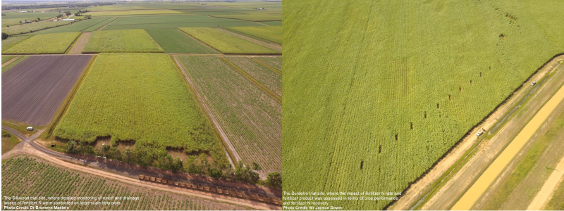
The dataset consists of tables of means, with statistical differences indicated where they are significant, for measured crop performance, fertilizer N recovery and use efficiency at 6 field sites from Mackay to Freshwater. Runoff losses of N are also shown from sites at Freshwater and Silkwood. **This dataset is currently under embargo until December 2021. Optimizing fertilizer nitrogen (N) application rates to both sustain high levels of productivity and minimize any impacts on the surrounding ecosystem is challenging, especially under monsoonal wet season conditions in northern Australia. The inability of existing application strategies and fertilizer N products to achieve synchrony of mineral N supply with crop demand, or prevent rapid formation of nitrate-N (that is vulnerable to loss via gaseous or aqueous loss pathways) increases risks of inefficient N use. A blend of enhanced efficiency fertilizers (EEFs) with different modes of action has the best chance of lowering the risk of N losses and increasing crop N recovery, providing an opportunity to reduce fertilizer N rates without increasing the risks of productivity loss. Six field trials were established from Mackay to the wet tropics, with data collected from consecutive ratoon crops at each site. Yields and indices of N use efficiency were developed for crops receiving urea-N at rates equivalent to that derived from the local SIX EASY STEPS guidelines, or as urea or a blend of EEF’s applied at N rates calculated using a block-specific yield target (PZYP) based on mill records. Laboratory and field trials conducted at the University of Qld to investigate the implications of fertiliser application in concentrated, subsurface bands on the efficacy of different EEF technologies relative to a granular urea standard supported the research in sugarcane fields. These application methods represent the current industry standard practice, but the band environment may adversely influence the rate of N release and/or subsequent N transformations that determine crop N uptake or environmental loss. Methods: The project established a total of six field sites after the 2016 crop harvest, with all experiments commencing after harvest of the 1st or 2nd ratoon. The experimental design and plot size varied with site. In Silkwood, Freshwater and the Burdekin, plots consisted of large scale strips 6-8 cane rows wide and the length of the cane block, with yield (and in the case of Silkwood and Freshwater, runoff water quality) collected from the whole treated strip. The Burdekin trial contained three replicate strips of each treatment, but due to the extensive water quality monitoring equipment requirements at Silkwood and Freshwater, treatments were not replicated. At all other sites, trials consisted of smaller plot, replicated experiments in a randomized block design. Plot size was at least 6 cane rows wide times 30m long, and all treatments were replicated four times. The basis of fertilizer rates was either the District Yield Potential (DYP, currently used to determine the fertilizer N rates in 6ES) or the Productivity Zone Yield Potential (PZYP, used to determine N rates aligned to a spatially relevant yield target). The PZYP was calculated from the mean yield from block or satellite records over two or more crop cycles, plus 2 times standard error of that mean. As all sites were established in ratoon crops, plant crop yields were generally excluded from this calculation, especially where those yields were markedly higher than yields of the ratoons. In situations where large variation in yields occurred between La Nina and normal or drier seasons (e.g. in the wet tropics), separate PZYP targets were calculated to reflect the expected seasonal forecast (i.e. lower PZYP targets in forecast La Nina conditions). Each site hosted a Nil N treatment each year (fertilizer N was withheld for that growing season), but these plots/strips were relocated to new plot/strip locations annually. Having the Nil N treatment always located on a plot with a history of fertilizer N application provided a realistic assessment of the soil N supply which the fertilizer N application was designed to augment. Crop harvest and fertilizer application were conducted as per grower normal practice at each location, although at all sites there were no crops harvested in the 1st round. This was considered desirable, as it was expected that the best chance to assess the risks of reduced N rates and the efficacy of EEF’s would be under conditions where fertilizer N losses were more likely to occur (i.e., where the onset of the monsoonal wet season occurred before the crop had finished the majority of biomass N accumulation). Fertilizer N sources The same fertilizer N sources were used at each site. The fertilizer N standard was taken as granular urea, which was applied during the month following harvest of the preceding ratoon. This was compared to an EEF blend consisting of 1/3 times urea coated with the nitrification inhibitor 3,4-dimethylpyrazole phosphate (DMPP, marketed commercially as Entec®) and 2/3 times polymer-coated urea with a reported 90-day release period (product of Everris Pty Ltd and marketed as Agromaster Tropical®). This blend was chosen as the best possible combination of products that would protect fertilizer N from risk of loss – initially by retaining the N in the NH4-N form, and subsequently by slowing the release of urea-N into the soil solution. Both products were applied using either stool-split (Burdekin, Freshwater, Mackay and Silkwood) or subsurface side-dress (Tully) fertilizer applicators, although it should be noted that on occasions the stool-split applicators did not always effectively close the fertilizer trench and cover the fertilizer band with soil. This suboptimal application strategy contributed to some confounding of the benefits of EEF use in some seasons due to greater loss risks to both the atmosphere and in runoff. Fertilizer N recovery, crop yield and indices of fertilizer N use efficiency Fresh and dry biomass and crop N content were determined from hand-cut biomass samples collected from 7-10 months after fertilizer application, on the assumption that at this stage, the crop N content would be at a maximum, and most relevant to the yield-determining processes. Crop N was partitioned between leaf/cabbage/dead leaf and stalks at that time. In situations where biomass sampling was conducted a little earlier than desirable (e.g. due to an impending cyclone), smaller numbers of whole stalk samples were again collected for dry matter and N concentration immediately prior to harvest (to determine the partitioning of N between harvested and non-harvested portions of the crop), and stalk N concentration from the final harvest was used in combination with cane yields to estimate crop N removal. Yields were determined by commercial harvest in the case of the large strip plots, with the bins collected from each strip weighed and ccs determined at the mill. In the case of the small plot trials, yields were determined from small plot hand harvesting and ccs was determined by near infrared spectroscopy. A number of indices of N use efficiency were calculated from these data including – -Agronomic Efficiency of fertilizer N use (AgronEffN) = Fertilizer N rate/(YieldN1 – YieldN0) = kg fertilizer N required to produce an additional tonne of cane yield. In this calculation, YieldN1 is the cane yield at fertilizer rate N1, while YieldN0 is the yield with no N applied. -Nitrogen uptake efficiency (NUpE) = (Crop N1 – Crop N0)/Fertilizer N rate = the additional crop N uptake/kg fertilizer N applied. In this calculation, N1 is the biomass N content for N rate 1, while N0 is the biomass N content with no applied N fertilizer. -Nitrogen Utilization Efficiency (NUtE) = Yield/Crop N content = t cane produced/kg of crop N uptake. This figure is a very useful indicator of trial sites where yield is constrained by factors other than N (e.g. waterlogging). Runoff and drainage losses of N Surface water runoff and drainage below the root zone (1 m depth) were monitored in four of the fertilizer rate treatments at Silkwood and Freshwater sites. In addition, strategic sampling in the farm drain around the Silkwood block was undertaken. Surface water samples were collected by automated samplers, with sampling undertaken across the hydrograph (Freshwater) or as an integrated composite of runoff from each individual runoff event (Silkwood). Runoff samples were analysed for sediment, total nitrogen, urea, ammonium-N, and nitrate-N (in addition to other constituents). Drainage samples were collected from 5 lysimeter barrels in each of the treatments with runoff monitoring (totalling 20 barrels) on a weekly to monthly basis at Silkwood. Drainage samples were analysed for nitrate-N and ammonium-N concentrations. Process studies of banded urea and EEFs A series of laboratory studies have been undertaken as part of a PhD program and subsequent short postdoc appointment to quantify the N dynamics relating to banded EEF’s (controlled release/coated products or stabilized products), due to concerns that the band environment may interfere with the operation of the EEF technology. This work has resulted in a series of publications that detail the key findings, but that also include supplementary data to provide background information. These papers are available from the NESP website. Limitations of the data: Data collectively represent variable soil types and seasonal conditions, so extrapolation from particular sites to other seasons, regions or soil types should be undertaken with extreme caution. Similarly, the performance of the EEF fertilizer blend used in this study is specific to the products used, and extrapolation to a broader range of EEF technologies would not be appropriate. This project played a key role in developing the research approach that was used in the Reef Trust 4 project EEF60 run by the Canegrowers organization, which represented a much broader testing of the combination of EEF fertilisers and reduced N rates on productivity and runoff water quality. Project scientists also set on the technical advisory group for that project. Format: The data from the field trial program consists of a series of spreadsheets containing crop summary data for each successive crop season at all sites. As of Jan 2021, the dataset is complete for 3 crop seasons at all sites and a 4th crop season at sites in Tully, Freshwater and Mackay. Data are presented as treatment means with statistical significance (P<0.05) indicated where appropriate. Due to the specific and controlled nature of the chemical assays of fertiliser N performance in bands, data is presented in detail in the technical publications and the related Supplementary material published with those manuscripts. These are available from the journal articles themselves, which can be assessed from the website. Similarly, there are a number of linked publications from research into the interaction between fertiliser application strategies and EEF technologies that were conducted at UQ Gatton, using maize as a test crop. NESP project 5.11 contributed to some of the analytical costs of this research (the trials were funded primarily by contributions from UQ and Kingenta Australia) where it complimented the NESP objectives, with that funding acknowledged in the manuscripts under development. However, the data does not relate to the core objectives of the project ‘Effects of fertilizer nitrogen (N) application rate and Enhanced Efficiency Fertilizers on sugarcane productivity, efficiency of N use and loss of N in runoff’, and so experimental data will not be provided in eAtlas. It will be reported in detail in the publications, as per the laboratory component. Data Dictionary: -EEF – Enhanced Efficiency Fertilizer. In the context of these trials, refers to a blend of 1/3 urea coated with the nitrification inhibitor DMPP (Entec ®) and 2/3 polymer coated urea (Agromaster Tropical ®) with a reported 90d release period. -Agronomic Efficiency of fertilizer N use (AgronEffN) = Fertilizer N rate/(YieldN1 – YieldN0) = kg fertilizer N required to produce an additional tonne of cane yield. In this calculation, YieldN1 is the cane yield at fertilizer rate N1, while YieldN0 is the yield with no N applied. -Nitrogen uptake efficiency (NUpE) = (Crop N1 – Crop N0)/Fertilizer N rate = the additional crop N uptake/kg fertilizer N applied. In this calculation, N1 is the biomass N content for N rate 1, while N0 is the biomass N content with no applied N fertilizer. -Nitrogen Utilization Efficiency (NUtE) = Yield/Crop N content = t cane produced/kg of crop N uptake. This figure is a very useful indicator of trial sites where yield is constrained by factors other than N (e.g. waterlogging). Data Location: This dataset is filed in the eAtlas enduring data repository at: data\custodian\2019-2022-NESP-TWQ-5\5.11_On-farm-nitrogen-management **This dataset is currently under embargo until December 2021

This project developed a set of high quality GIS datasets of the emergent and shallow marine features (reef boundaries, reef tops, islands, and cays) of the Coral Sea Marine Park (CSMP). The goal of this mapping was to improve the precision and spatial detail of existing reef maps. ## Features mapped: - Coral atoll platform boundary - outer visible extent (~40 - 60 m depth) - Coral reef boundary - coral substrate, plus connected sand, raised off atoll platform, mapped to 30 - 50 m depth. - Reef tops (5 m and 10 m depth) - Coral cays (above mean high water) - Coral cay vegetation - Beach rock - around coral cays and where visible on reef tops - Beach (high tide water to vegetation, excluding beach rock) - Structures (wrecks, weather stations, buildings) - incomplete coverage This project mapped reef boundaries features in a manner similar to the existing reef mapping of the Great Barrier Reef Marine Park (GBRMP) and Torres Strait (Lawrey, et al. 2016). The key characteristics of this mapping is the focus on determining the outer most boundary of coral reefs, where they rise up off the surrounding sea floor. In the Coral Sea the coral atoll platform was considered the sea floor and any solid coral structure raised up off the atoll platform was considered a coral reef. The reef boundaries also include sandy areas that connect close reef patches and surrounding sand that is highly connected to the coral substrate, as evidenced by halos (sand cleared of algae by fish around the coral patches). Patches of coral closer than 50 - 300 m were merged together to make fewer, but larger coral reef boundaries. The merge distance depended on slope, depth, structural uncertainty and visual uncertainty. The accuracy of the reef boundaries was checked by comparing digitisation of a subset of the features by independent team members. Digitised features were reviewed and refined by a second team member using additional imagery. Reef boundaries were linked with historic names based on nautical charts and historic maps, then assigned a permanent identifier that can be used instead of the reef name. Large reef features were cut into multiple segments where different sections are known by different names. In addition to reef boundary mapping the structure of the reef tops was mapped using satellite derived bathymetry to estimate a 5 and 10 metre depth boundary. The 5 m depth reef top aligns with the existing 'Dry reefs' mapping performed in the Great Barrier Reef. Shallow features were also mapped, including coral cays, surrounding beach rock and vegetation. Additionally the beach area (above high tide, but below vegetation) was mapped to provide a proxy for potential turtle nesting areas. Finally where they were visible, man made structures along with ship wrecks were mapped, however the resolution of the imagery available meant that these features were far from comprehensive. The features were digitised using a combination of satellite and drone imagery. Sentinel 2 (10 m resolution) and Landsat 8 (30 m resolution) imagery was used to map all marine features, drone imagery was used to map some of the cay areas, while the rest were mapped with publicly available ArcGIS World Imagery (~0.5 - 1m resolution). The Sentinel 2 and Landsat 8 imagery were processed into cloud free composite images using the Google Earth Engine. The imagery along with the processing scripts and mapped features are openly available.

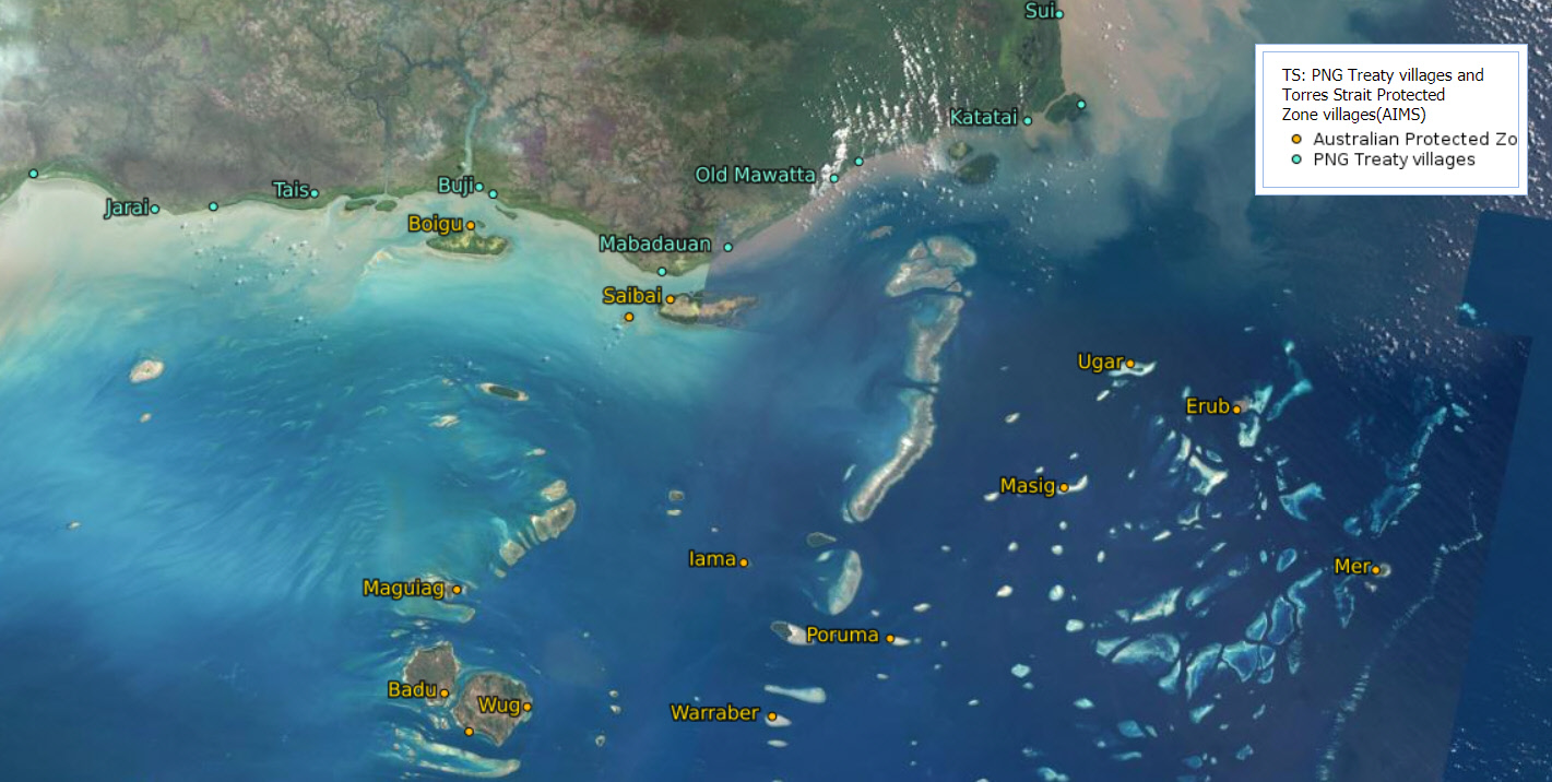
This dataset consists of a small CSV file containing the locations, names and country of the Torres Strait villages associated with the Australian and Papua New Guinea Treaty Protected Zone and neighbouring PNG Treaty villages This dataset is intended for the creation of regional maps. The village locations are not official and were based using satellite imagery to place the village marker on either the centre of the visible village, or the post office location, if that was marked in Google Maps. In 2000, Australia and PNG exchanged third person notes which identified the PNG villages deemed to be Treaty villages. Thus, PNG inhabitants from the 13 Treaty villages—Bula, Mari, Jarai, Tais, Buji/Ber, Sigabadaru, Mabadauan, Old Mawatta, Ture Ture, Kadawa, Katatai, Parama and Sui—can, without passports, visit the Protected Zone to carry out traditional activities. Torres Strait Islanders living in the Protected Zone have reciprocal rights to visit the Treaty villages to also carry out traditional activities. The spelling of the names of the villages were based on the maps and text provided on the Torres Strait Island Regional council website at http://www.tsirc.qld.gov.au/community-entry-forms/treaty-png-border-movements. This contains the villages locations for: Parama, Buji, Bula, Sigabadaru, Sui, Tais, Ture Ture, Ber, Kadawa, Katatai, Old Mawatta, Mari, Mabadauan, Jarai, Boigu, Badu, Poruma, Erub, Dauan, Arkai, Wug, Maguiag, Mer, Saibai, Ugar, Warraber, Iama, Masig Format: CSV file containing 28 rows and 4 columns (longitude, latitude, name, country) Data Dictionary: longitude, latitude: Decimal degrees of the village location. This was adjusted to be central to the village, or at the location of the post office if this was marked on Google Maps and it appeared to be a valid location. name: Name of the village with spelling based on the Torres Strait Regional Council website. country: Country that the village is in. Either 'PNG' or 'Australia' References: Torres Strait Regional Council (2016) Torres Strait Treaty & Border Movements. Accessed 12 April 2021 from http://www.tsirc.qld.gov.au/community-entry-forms/treaty-png-border-movements Senate Foreign Affairs, Defence and Trade Committee (2010) The Torres Strait: Bridge and Border. Senate Printing Unit, Parliament House, Canberra. https://www.aph.gov.au/Parliamentary_Business/Committees/Senate/Foreign_Affairs_Defence_and_Trade/Completed_inquiries/2010-13/torresstrait/report/index

This dataset is a compilation of available ocean temperature data, aerial and in-water bleaching observations during the 2016 and 2017 bleaching events on the Great Barrier Reef in order to estimate the total reef area impacted by coral bleaching and thermal heat stress. A total of 982 reefs (56.8% reef area of the GBR) were surveyed in 2016 and 781 reefs (50.9% reef area of the GBR) surveyed in 2017. This analysis provides an improved understanding of the variability and the increase in spatial impacts from coral bleaching throughout the GBR in a warming ocean. This data compilation of available bleaching survey data was used to provide: i) a quantitative assessment of the spatial variability of accumulated heat stress, severe coral bleaching and mortality throughout the GBR on regional and within individual reef scales, in comparison with previous widespread bleaching events in 1998 and 2002; ii) a quantitative comparison of bleaching observations from a range of observers which used a variety of methods and spatial assessments. The recent heat waves in 2016 and 2017 were unprecedented for the GBR. Temperatures remained above historical summer maximums for more than three months, and maximum anomalies in some locations were as high as 2.9°C (2016) and 3.2°C (2017) above the recent historical average summer maximum (1985-2012). During the 2016 - 2017 bleaching events, both coral bleaching and coral mortality occurred at a lower level of accumulated heat stress than previously proposed by the National Oceanic and Atmospheric Administration (NOAA) Coral Reef Watch (CRW) Degree Heating Week (DHW) product. The combined data recorded widespread coral bleaching occurring at a NOAA DHW value of 2-4 degree-weeks, severe bleaching, and some coral mortality at 5-8 DHW’s, and extensive mortality at reefs exposed to more than 8 DHW’s. Prior to this event, the general guideline based upon previous observations was that coral bleaching would occur at a DHW >4 and that coral mortality would begin at a DHW >8. In 2016 and 2017 on the GBR at heat stress exposures of 2.5°C-weeks we observed coral bleaching, after 5°C-weeks severe bleaching and some mortality and severe mortality following 8°C-weeks. Methods: All available aerial and in-water bleaching observations were assessed to quantify the relationship between coral bleaching and accumulated heat stress from ocean SST products and bleaching severity and coral mortality. Sea Surface Temperature Data was sourced from SSTAARS Climatology, NOAA-CRW Degree Heating Week (DHW). Broad spatial coverage of satellite Sea Surface Temperature (SST) monitoring products (NOAA Coral Reef Watch) were combined with the established relationship of observed bleaching severity with the accumulated heat stress product NOAA Degree Heating Weeks (DHWs), to scale up estimates of bleaching to the whole GBR. The NOAA Degree Heating Week product is a thermal stress index which combines the intensity of the temperature anomaly (Hotspot) at least 1°C above the historical summer Maximum Monthly Mean (MMM, Version 3.1) temperature (upper thermal threshold) with the duration of time exceeding this threshold over a 12 week period. Coral Bleaching Surveys Aerial Data was sourced from: Aerial – Berkelmans 1998 - Aerial survey of the GBR during the 1998 bleaching event [Region: Whole of GBR, Dates: 1998-03-09, Number of sites: 495 reefs]. AIMS Aerial – Berkelmans 2002- Aerial survey of the GBR during the 2002 bleaching event [Region: Whole of GBR, Dates: 2002-03-20, Number of sites: 1295 reefs]. AIMS Aerial - Hughes 2016 – Aerial survey of the GBR during the 2016 bleaching event [Region: Whole of GBR, Dates: 2016-03-22/2016-04-28, Number of sites: 924 reefs]. JCU and TSRA Aerial - Hughes 2017 – Aerial survey of the GBR during the 2017 bleaching event [Region: Whole of GBR, Dates: 2017-03-15 / 2017-04-05, Number of sites: 725 reefs]. JCU Aerial – AIMS 2017 - Aerial survey of the GBR during the 2017 bleaching event [Region: Townsville and Cairns, Dates: 2017-03-09, Number of sites: 70 reefs]. AIMS and GBRMPA Data handling: The data from Berkelmans 1998 and Berkelmans 2002 was presented with five-point rating (1-5) but converted to align with the Hughes dataset format (Category 0-4). Berkelmans Hughes 5 (<1% bleached) = 0 4 (1–10% bleached) = 1 3 (10–30% bleached ) = 2 2 (30–60% bleached) = 3 1 (>60% bleached) = 4 Methods: Aerial Bleaching Surveys: conducted from a combination of light fixed wing aircraft and helicopter, flying at an elevation of approximately 150m. This method accurately captures the proportion of healthy and bleached coral colonies in the shallow reef flat (0-3m) and in the upper reef slope (0-6m). Reefs were scored independently (isolated communications) by 2-4 observers looking out the left and right windows of the aircraft. Bleaching scores were recorded on spatial GBRMPA zoning reef maps, with mapping handheld GPS devices recording the flight path and confirming the reef location during the flight (Berkelmans & Oliver 1999; Berkelmans et al. 2004; Hughes et al. 2017). Surveys in 1998 and 2002, did not have GPS recorders. Reefs were categorised by visual assessment based upon the proportion of living coral visible to the observer that appeared bleached, severely bleached white, or fluorescent, into five community bleaching severity categories: 0 (no bleaching) <1%, 1 (moderate) 1-10%, 2 (high) 10-30%, 3 (very high) 30-60%, 4 (extreme bleaching) > 60%; These categories were used to align with the protocols developed in 1998 by Ray Berkelmans and GBRMPA (Berkelmans & Oliver 1999; Berkelmans et al. 2004). Photographs of each categorised reef in 2016 were recorded, stored, geo-located with GPS locations and made available to the public through the JCU Centre of Excellence for Reef Studies website (https://www.coralcoe.org.au/coral-bleaching-map). Images from the GBRMPA flight in 2017 between Townsville and Cairns will be available through the eAtlas. Coral Bleaching Surveys In-water: Sectors: • Far North (9-14°S; including the Torres Strait) • Northern (14-18°S; Innisfail to Cooktown) • Central (18-21°S; Mackay to Innisfail) • Southern sector (21-24°S; Mackay to Gladstone). AIMS 2016 - In water survey of reefs in the Townsville-Cairns area in 2016 [Region: Central and Northern sectors, Method: in water – 1m belt Transect, Dates: 2016-03-02 / 2016-04-06, Number of sites: 27 reefs] Reported metrics: Bleaching categories 1-4, % Mortality, % Bleaching AIMS 2017 - In water survey of reefs in the Townsville-Cairns area in 2017 [Region: Central and Northern sectors, Method: in water – 1m belt Transect, Dates: 2017-03-14 / 2017-04-01, Number of sites: 19 reefs] Reported metrics: Bleaching categories 1-4, % Mortality, % Bleaching GBRMPA 2016 - In water survey of reefs in the GBR area in 2016 [Region: all sectors, Method: in water – RHIS, Dates: 2016-03-02 / 2016-06-11, Number of sites: 102 reefs] Reported metrics: Bleaching categories 1-4, % Mortality, % Bleaching GBRMPA EotR 2015-2017- Eye on the Reef CoTS Control team observers in water survey of reefs in the GBR area in 2016/2017 [Region: all sectors, Method: in water – RHIS (5m radius), Dates: 2016-02-01 / 2017-04-30, Number of sites: 1200 reefs] Reported metrics: Bleaching percent by coral type, Mortality percent by coral type, % Bleaching, % Mortality Frade 2016 - Local survey up to 40m depth to test depth as refuge for bleaching. [Region: Far North and Northern sectors, Method: in water – 1m belt Transect, Dates: 2016-05-14/23, Number of sites: 6 reefs / 9 sites] Reported metrics: Bleaching categories 1-4. University of Queensland Global Change Institute. Baird 2016 - Local survey up to 27m depth to test depth as refuge for bleaching.[Region Far North, Method: in water – 1m belt Transect, Dates: 2016-04-11/14, Number of sites: 7 reefs / 11 sites] Reported metrics: Bleaching categories 1-6 to genus level coral ID Methods: In-water quantitative transect based surveys conducted by AIMS: In-water surveys were conducted between Townsville and Port Douglas by the AIMS at 54 sites within 19 reefs in 2016 and 40 sites within 12 reefs in 2017, from 13 March – 6 April 2016 and from 14 March – 1 April 2017. Surveys were conducted following the onset of maximum temperature exposure to capture the bleaching response at its peak, with an additional 0 – 2.9 DHW accumulating following the time of the survey. Follow up surveys were conducted in June 2016, September 2016 and September 2017 to assess survivorship. For each reef, surveys were conducted at three habitats: (1) shallow, sheltered reef flat at 2m; (2) exposed shallow reef slope at 3m; and (3) deeper exposed reef slope at 7-9m along permanent AIMS Long-term monitoring sites or equivalent on the northern exposed flank of each reef. Scleractinian hard corals >5cm in diameter were identified to genus level and bleaching severity categorised as: (1) healthy; (3) minor-moderate bleaching (paling/ 1-50%; (4) major bleaching (51-90% bleached); severe bleaching (100% white) and (6) recently dead (full colony or partial sections of the colony). In water surveys conducted by the University of Queensland Global Change Institute (Frade et al. 2018) were conducted between 14 - 23 May 2016 at nine sites within six outer shelf reefs in the Northern Sector of the GBR, at a depth of 5, 10, 25 and 40m, in order to determine the effect of bleaching over a large depth range. Surveys were conducted along 1m belt transects covering 75m length at each depth. Scleractinian hard corals >10cm in diameter were identified to genus level and bleaching severity categorised as: (1) healthy; (2) minor bleaching (paling/ 1-50%; (3) severely bleached (51-100% bleached) and (4) recently dead. In-water qualitative Reef Health Index Surveys (RHIS): In water surveys conducted by the GBRMPA field management team in 2016 were conducted at a total of 62 reefs across seven inshore-offshore transects following guidelines outlined in the Coral Bleaching Risk and Impact Assessment Plan (GBRMPA 2011). The survey plan aimed to conduct 15 or more Reef Health Index Surveys (RHIS) (that is, replicate samples) across three different locations on each reef, corresponding to three different aspects (north-east, north-west and south-west). At each of the western locations (i.e. north-west and south-west), three RHIS surveys were conducted at the same depth (approximately one to four metres), making a total of six RHIS. At the north-eastern location, three surveys were conducted at three different depths (approximately one to three metres, six metres and nine metres), making a total of nine RHIS. Surveys followed the standard protocol for Reef Health Impact Surveys (RHIS) (Beeden et al. 2014). Key information recorded includes: i) qualitative estimates of the percentage of the benthos (sea floor) made up by macroalgae, live coral, recently dead coral, live coral rock, coral rubble and sand; and ii) observations of coral impacts, and this is done over a series of five-metre radius point surveys (with one RHIS form completed for each circular plot of 78.5 square metres). The percentage of coral cover (if any) that had recently died from each impact-type (that is, bleaching, disease, predation, damage) was estimated as described in Beeden et al. (2014) for each RHIS survey by examining all coral colonies within the point surveys for any impacts. These data were used to categorise the percentage of bleached corals within the total living coral within each RHIS area. For comparison to all aerial survey data and the in-water transect based quantitative estimates, the average RHIS per cent bleached scores for each reef were converted to align with the aerial bleaching categories described above (Berkelmans et al. 2004). In-water surveys conducted by the COTS Targeted Control Program were also collected for this analysis from the Eye on the Reef Program from 2016 and 2017 (RRRC and AMPTO 2016). Three RHIS surveys were conducted at each reef and followed the standard protocol for RHIS (Beeden et al. 2014), recording the percentage of bleached corals among the living coral cover in addition to records of coral cover, coral type and potential COTS presence, absence and damage. Bleached corals were categorised according to the GBRMPA Coral Bleaching Response Plan (GBRMPA 2011) among four RHIS Colony bleaching levels: (1) upper surfaces (2) Pale/Fluoro (3) Totally white (4) Recently dead. Data handling: All in-water bleaching observations were converted to align with the National Bleaching Taskforce aerial bleaching categories 0-4. For community level bleaching response transect and RHIS based observations were converted into a percentage (%) bleached of all corals counted from the survey method, which was then converted into the 5 category scale used by the aerial survey scores. The in-water and aerial bleaching observations to establish the relationship between total heat stress accumulation (DHW) and the overall coral community level bleaching response (% of living corals bleached) were combined. The in-water transect and RHIS were combined to provide estimates of the proportion of individual coral colonies that were severely bleached or recently dead. Further information can be found in the report: Cantin, N. E., Klein-Salas, E., Frade, P. (2021) Spatial variability in coral bleaching severity and mortality during the 2016 and 2017 Great Barrier Reef coral bleaching events. Report to the National Environmental Science Program. Reef and Rainforest Research Centre Limited, Cairns (64pp.). Format: GIS Spatial layers, Tif and KML files. Data Dictionary: GBR Community Bleaching Surveys - over the 2016-2017 time frame 0 (<1% bleached) 1 (1–10% bleached 2 (10–30% bleached ) 3 (30–60% bleached) 4 (>60% bleached) GBR: NOAA Coral Reef Watch – GBR Maximum Monthly Mean (MMM; raster) - Historical average maximum of the monthly mean temperatures for 1985-2012 climatology (v3.1) from annual sea surface Temperature anomalies. Represents the upper thermal limit for each location. 25 °C 26 °C 27 °C 28 °C 29 °C 30 °C GBR: NOAA CRW – DHW max [2002, 1998, 2016, 2017] Maximum accumulation of Degree Heating Weeks for each bleaching year. The NOAA DHW product is a summation of temperature anomalies at least 1°C above the MMM value over a 12 week period, which generates a measure of thermal stress as a function of both the strength of the anomaly above the MMM and the duration of the heating event. The DHW max value used here is the maximum DHW value accumulated for each summer heat wave. 0 °C – weeks 2 °C – weeks 5 °C – weeks 8 °C – weeks 15 °C - weeks References: Beeden R, Turner M, Dryden J, Merida F, Goudkamp K, Malone C, Marshall Paul A, Birtles A, Maynard J (2014) Rapid survey protocol that provides dynamic information on reef condition to managers of the Great Barrier Reef. Environmental Monitoring and Assessment 186:8527-8540 Berkelmans R, Oliver JK (1999) Large-scale bleaching of corals on the Great Barrier Reef. Coral Reefs 18:55-60 Berkelmans R, De'ath G, Kininmonth S, Skirving W (2004) A comparison of the 1998 and 2002 coral bleaching events on the Great Barrier Reef: spatial correlation, patterns and predictions. Coral Reefs 23:74-83 Cantin, N. E., Klein-Salas, E., Frade, P. (2021) Spatial variability in coral bleaching severity and mortality during the 2016 and 2017 Great Barrier Reef coral bleaching events. Report to the National Environmental Science Program. Reef and Rainforest Research Centre Limited, Cairns (64pp.). Frade PR, Bongaerts P, Englebert N, Rogers A, Gonzalez-Rivero M, Hoegh-Guldberg O (2018) Deep reefs of the Great Barrier Reef offer limited thermal refuge during mass coral bleaching. Nature Communications 9:3447 GBRMPA (2011) Coral Bleaching Response Plan. Great Barrier Reef Marine Park Authority, Townsville Hughes TP, Kerry JT, Álvarez-Noriega M, Álvarez-Romero JG, Anderson KD, Baird AH, Babcock RC, Beger M, Bellwood DR, Berkelmans R, Bridge TC, Butler IR, Byrne M, Cantin NE, Comeau S, Connolly SR, Cumming GS, Dalton SJ, Diaz-Pulido G, Eakin CM, Figueira WF, Gilmour JP, Harrison HB, Heron SF, Hoey AS, Hobbs J-PA, Hoogenboom MO, Kennedy EV, Kuo C-y, Lough JM, Lowe RJ, Liu G, McCulloch MT, Malcolm HA, McWilliam MJ, Pandolfi JM, Pears RJ, Pratchett MS, Schoepf V, Simpson T, Skirving WJ, Sommer B, Torda G, Wachenfeld DR, Willis BL, Wilson SK (2017) Global warming and recurrent mass bleaching of corals. Nature 543:373-377 Data Location: This dataset is filed in the eAtlas enduring data repository at: data\nesp5\5.7_Bleaching-Assessment