This record provides an overview of the NESP Marine and Coastal Hub study - Assessing dugong distribution and abundance in the southern Gulf of Carpentaria. For specific data outputs from this project, please see child records associated with this metadata. Aboriginal ranger groups, Traditional Owners of the southern Gulf of Carpentaria (sGoC), scientists, Queensland, Northern Territory and Commonwealth government representatives will co-design and implement a program that enables a contemporary cross-border understanding of dugong populations and other marine megafauna. The dugong program comprises three parts: 1) Dugong population genetics, 2) a standardised aerial survey in the sGoC, and 3) Indigenous-led drone surveys of marine megafauna hotspots. The collaborative approach will enable contemporary data on abundance, distribution and genetic population structuring to inform local and regional conservation management actions. In combination with other NESP investments in Qld and WA, this program will have applied consistent approaches to dugong population assessment across three states. This program directly responds to the national priorities of conserving, protecting and sustainably managing biodiversity through research and information management. Planned Outputs • dugong distribution & abundance [spatial dataset] • Final technical report with analysed data and a short summary of recommendations for policy makers of key findings [written]

This record provides an overview of the NESP Marine and Coastal Hub study - Scaling-up long-term seagrass restoration in the Cocos (Keeling) Islands. For specific data outputs from this project, please see child records associated with this metadata. There is an urgent community-driven need to develop appropriate seagrass restoration approaches at scale for the Cocos (Keeling) Islands (CKI). Fast-tracking larger-scale restoration research is required to prevent imminent collapse and functional extinction of seagrasses at CKI due to past disturbance and current green turtle grazing pressure. This project builds on pilot studies to design and establish a network of larger-scale turtle exclusion areas where locally appropriate restoration approaches can be refined. At the same time, this will provide “seagrass refuges” to initiate recovery, monitor ecological effects, and provide for future restoration efforts. The project has been co-developed with the CKI community and Parks Australia, addressing their highest research priority identified in the newly established Cocos (Keeling) Islands Marine Park. The project will provide an action plan for ongoing interventions and strategies to future-proof local seagrasses and support seagrass-dependent species, such as green turtles and fish, in the long term. Planned Outputs • exclusion zones experimental data [spatial & tabular dataset] • environmental monitoring dataset [tabular data] • Final technical report with analysed data and a short summary of recommendations for policy makers of key findings [written]

This record provides an overview of the NESP Marine and Coastal Hub study - Developing Traditional Owner community-led dugong monitoring in the Kimberley region. For specific data outputs from this project, please see child records associated with this metadata. Dugong are a keystone species with considerable ecological and cultural value across northern Australia. In the Kimberley region of Western Australia, dugongs have been identified as one of the top priorities to monitor in an effort to ensure the population is maintained and traditionally harvested in a sustainable manner. This project aims to have Traditional Owners and ranger groups across the Kimberley use cost-effective and culturally appropriate approaches to (1) fill knowledge gaps on the dugong’s population structure and connectivity at a range of spatial and temporal scales and (2) monitor the animals’ presence, density and habitat use in areas that are ecologically and culturally important to the local community and state and federal managers. This program directly addresses the national priorities of conserving, protecting and sustainably managing biodiversity through research and information management. Planned Outputs • dugong distribution and abundance [spatial dataset] • aerial survey outputs [imagery & photogammetry] • genomic sequencing data • code and scripts • Final technical report with analysed data and a short summary of recommendations for policy makers of key findings [written]

This record provides an overview of the NESP Marine and Coastal Hub project 'Towards assessing the values of reefs in the southern Gulf of Carpentaria 2024 - 2025'. For specific data outputs from this project, please see child records associated with this metadata. The Gulf of Carpentaria Marine Park was only recently declared in 2013. The zoning plan for this marine park, which permits trawling within a specific trawling zone is due for renewal by 2028. There is a strong need to collect, analyse, synthesise and make publicly available information on the values and conditions of key habitats within the Marine Park, such as recently identified patch reefs and coral reefs, to contribute to this upcoming review of the management plan for this marine park. The limited scientific information that is available on the values of this marine park is hard to access and much of it has not been analysed or written up. In addition, the Traditional Owners hold much valuable information about the ecological and cultural values that should inform future park management decisions. This project aims to gather, synthesise and report on existing scientific data and information about coral and patch reefs in the marine park. This information will be presented to the Traditional Owners and other relevant stakeholders at community meetings or workshops. Documenting cultural values of the reefs in this marine park is beyond the scope of the current project and would require considerable further engagement with Traditional Owners. However, it is anticipated that presentation of existing scientific and biophysical data at community meetings will start this process. We will produce visual (e.g. photos and videos) outputs that illustrate the values of these reefs, in order to better inform stakeholders involved in decisions about future park management. Planned Outputs • Final technical report with analysed data and a summary of recommendations for policy makers of key findings [written]

This record provides an overview of the NESP Marine and Coastal Hub project 'Supporting recovery and management of migratory shorebirds in Australia'. For specific data outputs from this project, please see child records associated with this metadata. Coastal Australia is home to 37 regularly occurring migratory shorebird species, with many protected areas including Ramsar sites designated on the basis of shorebird populations. Many migratory shorebirds are declining rapidly, and hence the focus of conservation efforts at multiple levels of government in Australia and overseas. Excitingly, after decades of decline, many of Australia’s migratory shorebird populations are now showing improving trends (NESP MaC Project 1.21 - Australia’s Coastal Shorebirds: Trends and Prospects). However, we do not understand why the birds’ populations are stabilising, or how these gains can be converted into genuine population recovery to previous population levels. This project will combine analyses on more than a million observations of shorebirds banded in Australia with a comprehensive database of management actions to (i) create an annually updatable dashboard providing the key shorebird population parameters of reproductive output and survival, (ii) build a comprehensive database of conservation management actions for migratory shorebirds, indicating which actions are known to benefit reproductive output and survival, and (iii) create a shorebird management handbook that can be used by practitioners to guide action across Australia and around the East Asian – Australasian Flyway. Outputs will support DCCEEW’s international obligations in relation to Ramsar wetlands, the Convention on the Conservation of Migratory Species (CMS), bilateral migratory bird agreements with Japan (JAMBA), China (CAMBA) and the Republic of Korea (ROKAMBA) as well as feed directly into developing the new incarnation of the Australian Government’s Wildlife Conservation Plan for Migratory Shorebirds. Results have a pathway for regional and local implementation through BirdLife Australia’s Migratory Shorebirds Conservation Action Plan. Planned Outputs • Annually updateable dashboard providing estimates of reproductive output and survival • Searchable database of conservation management actions for migratory shorebirds • Shorebird habitat management handbook that can be used by practitioners • Final technical report with analysed data and a short summary of recommendations for policy makers of key findings [written]

This record provides an overview of the NESP Marine and Coastal Hub study - Protecting valuable shoreline mangroves of northern Australia. For specific data outputs from this project, please see child records associated with this metadata. The mass death (~80 km2) and dieback of shoreline mangroves around the Gulf of Carpentaria (GOC) and across northern Australia in 1982 and 2015 was a wake-up call to the vulnerability and immense importance of marine coastal ecosystems like mangroves. It is essential that we fully understand the circumstances surrounding such catastrophic events, the environmental triggers identified, and what we might do to restore the damage while also preventing future occurrences. In response to the 2015 mass dieback event (the world’s largest such recorded event), the NESP commissioned an Emerging Priority project that utilised aerial surveys to assess the extent of the dieback along the entire Gulf of Carpentaria coastline. It is proposed to resurvey GOC shorelines for their current condition whilst taking the opportunity further to devise a well-considered and fully costed rapid response plan that will include innovative preventative management outcomes for the longer-term sustainability of threatened but highly-valued coastal marine ecosystems of northern Australia. Planned Outputs • aerial survey imagery [imagery] • satellite imagery analysis [spatial dataset] • field & environmental surveys [tabular dataset] • Final technical report with analysed data and a short summary of recommendations for policy makers of key findings [written]

Vegetation and Elevation surveys were conducted at four sites in the Gulf of Carpenteria to provided crucial validation of observations made from aerial surveys and provided further significant insights of the impacts and subsequent changes that occurred across the Gulf coastline up to late 2019. Field studies primarily focused on shoreline fringing stands dominated by the Grey Mangrove Avicennia marina var. eucalyptifolia. A total of eight transects, perpendicular to the shoreline were established at four shoreline sites across the Gulf of Carpentaria. These included matched pairs for each of two severity levels of 90%–100% and 60%–80% dieback of mangrove fringes. A series of profile transects were established and measured from the landward edge to the sea edge of mangroves. Transects were run from a highwater point at the head, directly towards the sea edge. This method captured common reference elevation levels for all sites while maximising coverage of the entire elevation range of the tidal wetland (mangroves plus tidal saltpan and saltmarsh vegetation), from approximately highest astronomical tide levels (~HAT) at the head, to approximately mean sea level (~MSL) at the seaward edge of living mangrove trees. On ground surveys consisted of two components: a) elevation measures from HAT (highest astronomical height – defined by the highwater mark) to MSL (mean sea level – defined by the seaward mangrove edge); and b) vegetation species, structure and density for mangrove and saltmarsh species present along with observations of condition and being likely 2015 dieback. The latter condition was determined from vegetative degradation states of mangrove trees, and as seen in satellite imagery mapping. Methods: Locations: The field studies started with the two locations in Queensland during 4–10 August 2018 and then moved onto those in the Northern Territory during 11–17 October 2018. A total of eight transects, perpendicular to the shoreline were established at the four shoreline sites across the Gulf of Carpentaria. Limmen – Roper region (NT) - 1A with 90% - 100 % dieback - 1B with 60% - 80% dieback Mule - Roper region (NT) - 2B with 90% - 100 % dieback - 2A with 60% - 80% dieback Karumba - SE Gulf (QLD) - 4A with 90% - 100 % dieback - 4B with 60% - 80% dieback Mitchell north - W Cape (QLD) - 5A with 90% - 100 % dieback - 5D with 60% - 80% dieback Transect Set Up Summary: Each transect was based or anchored at the observed nominal Highest Astronomical Tide (~HAT) level of the highwater benchmark at each transect ‘head’, via the beach wash zones indicative of the highest reach of tidal waters. A second reference position at the sea edge of mangroves was taken as a proxy relative to mean sea level (~MSL). The location of the head position was chosen so that a straight line transect could be taken to the fringing mangrove stand, and to the sea edge at the proxy position of mean sea level (~MSL). Three additional ‘internal’ ecotone position markers between ~HAT and ~MSL of the tidal wetland zone were recorded for each transect, including the landward fringing mangrove to the saltpan–saltmarsh position (M1-lower); the lower elevation limit of saltpan–saltmarsh bordering the upper dieback mangrove edge (M2-upper); and the lower elevation limit of mangrove dieback (M2-dead/live). Further details about the transect set up can be found in the final report volume 2 (Duke et al, 2020). Surveys: Long plots were used to describe and quantify mangrove and saltmarsh vegetation along each transect. The long plot method allowed the plot width to be adjusted during the survey depending on stem density of particular sections along the transect - where there were closely spaced trees, plots were narrower (<2 m wide) than where trees were larger and further apart (>2 m wide). Elevation levels were recorded at 20–30 m intervals or more frequently where there were otable changes in topography or there were notable changes in vegetation type and condition. Levels were made using a Topcon construction surveyors rotating laser and staff. Where it was necessary to relocate the laser instrument, additional reference points were taken for each transition point providing offset measures to link each series of measurements. Elevation levels were recorded all the way from the head marker to the sea edge amongst or just beyond the last trees. Vegetation was scored for species, stem diameter, height, condition as well as distance along the transect and distance left or right of the measuring tape. Trees were scored in 30 m sections within a fixed distance from the measuring tape depending on stand density. The width was mostly set at two metres, but on occasion, this was reduced to one metre or up to four metres wide as necessary. Along each transect, at each 30-metre interval or at ecotone points, photographs were taken at four square directions to the transect line – towards the sea, 90 degrees to the right, back towards the ‘head’ and 90 degrees to the left. At these same points, canopy photos were taken using a camera with a fisheye lens. The survey data contains wood sampling and tree coring investigations which could not be completed during the project's reporting time frame. Future project work will include high-level analytical work required, including elemental scans and carbon dating. Evidence of tree cores collected during the field surveys can be found within each vegetation survey sheet and the tree cores tab of the workbooks. Limitations of the data: While terrestrial forestry practice recommended that stem diameter be measured at 1.3 m above the ground – as diameter measured at breast height (DBH) – this was found to be impractical in these and other mangrove forests. The difficulties encountered included the common occurrence of multiple stems, short height mature trees and shrubs (<1.3 m), multiple forms of plant types (shrubs and trees), low branching (<1.3 m), and high placed roots and buttresses (>1.3 m). A more appropriate standard was applied in these studies of measuring stem diameters above highest prop roots and buttresses and below lowest branching Special consideration was taken in measuring stem diameters because slight differences in these measures could create considerable differences and errors in calculations of biomass and carbon content when using allometric equations. Format of the data: The data are complied in two excel workbooks detailing the QLD and NT surveys. The workbooks contain three tabs for each survey type (Vegetation transect data, transect elevation profile and undercanopy surveys). Both workbooks contain a Totals/Summary tab with statistics from each site, as well as a tree cores tab detailing the core samples. Data dictionary: see data package For the map layer: LOCATION: Name of the site HEAD_LAT: Latitude of the transect head point in decimal degrees HEAD_LONG: Longitude of the transect head point in decimal degrees SEAWARD_LA: Latitude of the transect head or seaward point in decimal degrees SEAWARD_LO: Longitude of the transect head or seaward point in decimal degrees IMPACT_SEV: Whether the site is a high dieback or moderate dieback site LENGTH : Length of the transect in meters ELEVATION: Elevation range in meters (m) CANOPY_DOM: Dominate species of tree for the transect P__DEAD_CA : Percent of dead trees in the canopy survey. Recorded in the % Damage (tree loss) cell at the top of each vegetation survey tab. The total live and dead trees are calculated, then summed to show the total survey trees. The equation of total dead trees/total trees*100 is used to them present the % damage (tree loss) figure. TOTAL_CANO: Shows the total number of live and dead trees in the transect MAX_CANOPY: Records the tallest tree surveyed in the transect (uses MAX formula in each Vegetation TREEs datasheet) UC_DOM__SP: Records the dominate undercanopy speecies, found on each site Undercanopy tab - columns Live & dead: AM Sap / AM Seedl, AA shrub/ AA seedl, Other Sap Species, Other Seedl species P__DEAD_UC : Percent of dead growth in the undercanopy. From the undercanopy tab of each transect fite, the total counts of live and dead Sap / Seedl are calculated for each species, then totalled in UC Live, UC Dead. The % Dead UC then uses equation of total dead UC/Total UC*100 to present the % UC Dead figure. TOTAL_UC: Records the total UC figure (total counts of live and dead Sap / Seedl are calculated for each species) MEAN_UC_HG: Mean height of the undercanopy in meters (m) TREE_CORES: Number of tree cores for the transect MEAN_STEM: The mean steam diameter (cm) for the transect References: Duke N.C., Mackenzie J., Hutley L., Staben, G., & Bourke A. 2020. Assessing the Gulf of Carpentaria mangrove dieback 2017–2019. Volume 2: Field studies. James Cook University, Townsville, 150 pp. eAtlas Processing: The original data were provided as two excel workbooks. No modifications/ minor modifications to the original data were performed. This metadata was created using the above referenced report. The map layer is derived of summary data extracted from the workbooks. Included in the data download package is our best estimate of the descriptions for the data attributes as a draft data dictionary which will be updated when further information is made available by the project team. Location of the data: This dataset is filed in the eAtlas enduring data repository at: data\\custodian\2018-2021-NESP-TWQ-4\4.13_Assessing-gulf-mangrove-dieback

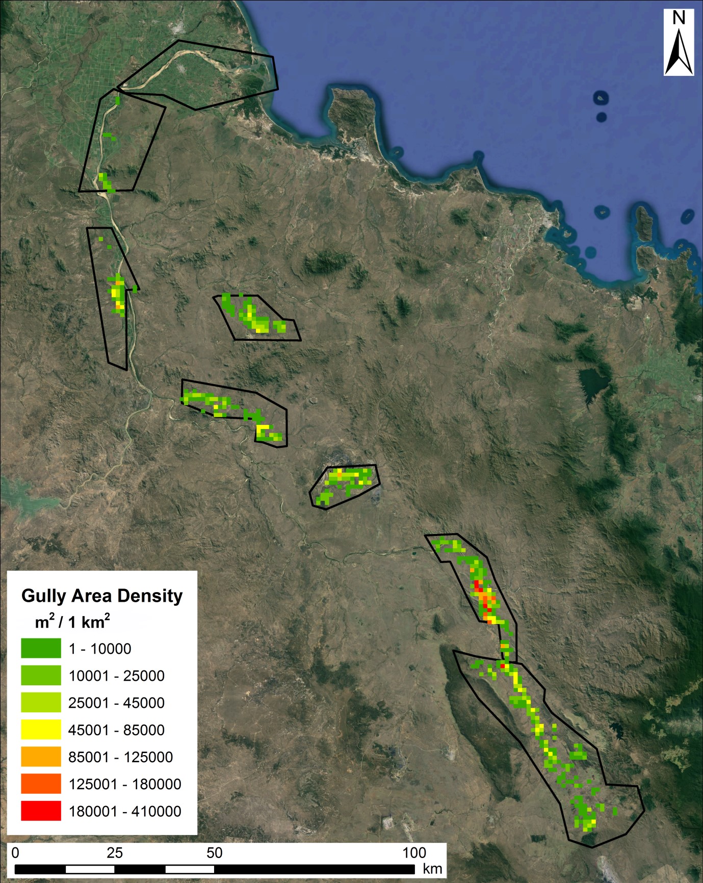
This dataset contains maps of alluvial and hillslope gullies across blocks of lidar covering portions of the Burdekin Catchment. This project is an expansion of the detailed gully mapping and assessment undertaken previously as part of NESP TWQ Project 5.10 (Daley et al., 2021), using newly available lidar as well as some older data not previously used. The gully polygons were generated using methods developed in the NESP TWQ 5.10 project for the extraction of gullies from lidar. Lidar is detailed topographic data collected from aircraft using an airborne laser scanning system. Methods: Lidar mapping and Gully Assessment SON3352211, December 2023. This project should be considered as the first step of a ‘prospecting’ effort, whereby high yielding high priority gullies are identified. Further investigations will be required (including on ground inspection) to firm up the prioritisation of gullies for rehabilitation. In all, gully mapping has been conducted across 1625 km2 (Figure 1). This is the area of lidar derived DEMs adjoining the areas within the Burdekin previously analysed by Daley et al. (2021) (Figure 1). This report briefly describes the generation of a new gully mapping dataset covering the 8 lidar blocks of the study area. Daley et al. (2021) provide a comprehensive description and discussion of the methods used below. Two small departures from the methods outlined therein have been adopted here. Firstly, the production of data layers was reordered, such that analyses that were previously restricted to just areas mapped as eroded landforms (i.e. PAE and Bare Soil described below) were here undertaken across the whole landscape, with the presence of high values for these metrics being used to identify areas for further investigation. This is a reversal (in a sense) of the approach used by Daley et al, who mapped all “gully like” features and then used PAE and Bare Soil metrics to distinguish actual gullies from features merely gully like. Here the approach has been to only search for (and map) gullies within areas of high PAE and Bare Soil. The second difference adopted here has been to define gully boundaries using two separate techniques for all observed gullies. In Daley et al, the choice of technique used to define the gully boundary was based on interrogation of general landscape slope, with 2% selected as a threshold separating areas where the Multi-direction hillshade (MDHS) approach was used from areas where the Mean Digital Elevation Model of Difference (Mean DoD) method was used. Early experimentation as part of this project found that this threshold method was occasionally unsatisfactory, as there were instances across all slope classes where the alternative approach provided the better representation of gully outline. In general, it was found that the MDHS method worked best where the gully had a more open form, which generally, but not always, occurred in areas of lower slope. Likewise it was found that the Mean DoD method worked best for linear or more reticulated forms, which generally but not always occurred in areas of higher slope. Examples of where the later did not apply is when an open form gully has mostly stabilised and revegetated, then re-incised, with the early phases of this re-incision taking the form of inset, more or less linear and/or reticulated gullying. To avoid the large amount of manual editing required where an inappropriate method was applied, it was found to be more parsimonious to run both techniques across all gullies, then select the approach which provided the best definition of gully boundary, requiring the least amount of manual digitising. 1. Mosaiced Digital Elevation Models (DEM) One kilometre square DEMs were obtained from Geoscience Australia’s ELVIS portal (https://elevation.fsdf.org.au/) and mosaiced into 8 larger DEMs, each covering one of the 8 non-contiguous areas shown in Figure 1. The DEM data was used to define gully margins and derive the Potential Active Erosion (PAE) layers. As depicted in figure 1, the spatial resolution of the DEMs of blocks 1 to 5 is 0.5 m and blocks 6 to 8 is 1 m. 2. Potential Active Erosion (PAE) The PAE method developed (and wholly described) by Daley et al. 2021 is an index of landscape curvature or crenulation. The index uses a measure of surface roughness derived using a log-transformed standard deviation of terrain curvature. Most erosion activity indicators correspond to areas exhibiting high values of surface roughness, including fluting, rilling, block collapse, slumping and exposed tree roots. As erosion activity decreases, slopes relax to more diffuse forms with lower roughness. Terrain roughness was measured as the local standard deviation of curvature in a 3 m kernel window, assessed from total, plan and profile curvatures. As roughness was highly skewed, with most values approximating zero, the data was log-transformed for ease of interpretation. Planform, profile and total curvatures were calculated within a 9-cell (3 x 3 m) neighbourhood using the ArcGIS curvature tool following the method of Moore et al. (1991) and Zevenbergen and Thorne (1987). All three types of curvature were evaluated to generate roughness indices following current literature as the log-normalised standard deviation of curvature (Korzeniowska et al. 2018; Patton et al. 2018). As standard deviation values in a 3 m cell kernel size were strongly right skewed, values were transformed using a base-10 logarithm function to normalise the distribution for ease of interpretation. Following Daley et al., a threshold log-normalised standard deviation of curvature value of 1.8 was chosen to define areas of PAE. 3. Bare Soil Baresoil was determined using PlanetScope Analytic data, with all scenes collected soon after the end of the 2022-2023 wet season. PlanetScope provides 4-band multi-spectral ortho scene data for analytic and visual applications. The provided product is orthorectified, radiometrically calibrated into top-of-atmosphere radiance data and then atmospherically corrected to surface reflectance, resampled to 3 m (Planet Team, 2020). This data was specifically selected for 90% coverage in a given acquisition. Additional data from neighbouring days were selected to fill in any gaps for complete coverage. Following data acquisition, scenes were mosaiced in a GIS to provide a continuous coverage dataset across the 8 study areas. Bare soil was derived from the PlanetScope imagery using the modified secondary soil-adjusted vegetation index (MSAVI2), Qi et al. (1994). MSAVI2 was selected as the most appropriate vegetation index for the region for its capacity to separate vegetation signatures in areas where vegetation cover is low, or features a high degree of exposed soil surface, and has the benefit over other soil-adjusted vegetation indices in that it does not require the calculation of a soil-brightness correction factor. MSAVI2 was developed iteratively by Qi et al. (1994) to determine the per-pixel difference of the red band reflectance value against the near infrared band, using the following equation: MSAVI2 = (2×NIR + 1 - √((2×NIR+1)^2 - 8×(NIR-RED)))/2 This yields an output of vegetation greenness with values ranging from -1 to +1. Following Daley et al, a threshold of 0.35 was used to identify bare soils. 4. Gully Mapping Gully boundaries were produced using the aforementioned Multi-direction hillshade (MDHS) and Mean DEMoD automated geomorphic mapping algorithms. For MDHS, the hillshade tool in ArcGIS Spatial Analyst is used iteratively, with the sun angle set at 15 degrees and passed through the six azimuths (0, 60, 120, 180, 240, 300 degrees). The output rasters of the hillshades are then mosaiced and areas <= 55 (i.e., lowest greyscale intensity value) are selected. These values are generally a function of slope and aspect for any given cell, but in this case, they are viewed as the amount of shadow generated by the moving sun. At each azimuth, the boundary of an eroded land form (ELF) is shadowed perpendicular to the direction of light. By merging the six hillshades, the boundary of a given gully is accurately extracted (see cross section C in Figure 2). In certain instances when a feature has low or diffuse walls, or a broad floor, the centre of the gully may not be shadowed, hence the centre of these gullies are filled to create a clean boundary. The Mean DoD method identifies abrupt changes in elevation assuming such changes equate to steep slopes on the walls of gullies. The mean focal statistic function was used with a circular window having a kernel radius of 25m. 5. Gully Distribution The area covered by the gully mapping polygons was divided into a 1 km x 1 km grid. One or two square kilometres is assumed to represent the size of an area that could be managed as one site containing multiple gullies. For each polygon the total area of mapped gullies contained within has been calculated (Figure 4) and plotted as a heat map. This is to facilitate prioritisation based on combined gully area within close proximity, rather than based on the size of any single gully. Limitations of the data: The funding for this project necessitated different priorities and a different scope of works than that of NESP TWQ 5.10, and consequently the set of derived gully metrics in this project is a subset of those in NESP TWQ 5.10. This dataset is specifically a selection of large prospectively high yielding gullies mapped as preparatory work towards future landscape repair programs which require detailed maps of gully extent in order to enable prioritisation and planning of works. This project should be considered as the first step of a ‘prospecting’ effort, whereby high yielding high priority gullies are identified. Further investigations will be required (including on ground inspection) to firm up the prioritisation of gullies for rehabilitation. Format of the data: Two shapefiles The gully mapping dataset consists of the shapefile – ‘Gully Mapping - Project SON3352211.shp’. The shapefile contains 1713 gully polygons. The gully density dataset consists of the shapefile – ‘Gully Density One km Grid - Project SON3352211.shp’. The shapefile contains 467 one km grid square polygons. Data dictionary: Gully mapping shapefile (Gully Mapping - Project SON3352211.shp) attribute table fields X - X co-ordinate of gully polygon centre point Y - Y co-ordinate of gully polygon centre point Gully_Code - Gully polygon ID number BaseData - DEM data acquisition name as stored in Geoscience Australia’s ELVIS data portal CellSize - Raster cell size (m) of base DEM data G_Area_m2 - Gully polygon area (m2) BS_Area_m2 - Area of bare soil as derived from Planet Scope imagery (m2) within gully polygons PCT_BS - Bare soil area as percentage of gully polygon area PAEArea_m2 - Area of Potential Active Erosion (m2) within gully polygon PCT_PAE - Potential Active Erosion area as percentage of gully polygon area Gully density shapefile (Gully Density One km Grid - Project SON3352211.shp) attribute table fields X - X co-ordinate of one km grid square polygon centre point Y - Y co-ordinate of one km grid square polygon centre point GulArea_m2 - Area of gully polygon within one km grid square (m2) References: Daley, J., Stout, J.C., Curwen, G., Brooks, A.P. and Spencer, J. (2021) Development and application of automated tools for high resolution gully mapping and classification from lidar data. Report to the National Environmental Science Program. Reef and Rainforest Research Centre Limited, Cairns (169pp.). Korzeniowska, K., Pfeifer, N., & Landtwing, S. (2018). Mapping gullies, dunes, lava fields, and landslides via surface roughness. Geomorphology, 301, 53-67 Moore, I.D., Grayson, R.B., Landson, A.R. (1991) Digital Terrain Modelling: A Review of Hydrological, Geomorphological, and Biological Applications. Hydrological Processes 5: 3–30. Patton, N. R., Lohse, K. A., Godsey, S. E., Crosby, B. T., & Seyfried, M. S. (2018). Predicting soil thickness on soil mantled hillslopes. Nature communications, 9(1), 3329. Planet Team (2020). Planet Imagery Product Specification. San Francisco, CA. https://developers.planet.com/changelog/2020/Jun/17/imagery/2020-06-17/ Qi, J., Chehbouni, A., Huete, A.R., Kerr, Y. H., and Sorooshian, S. (1994). A Modified Soil Adjusted Vegetation Index. Remote Sensing of Environment. 48: 119-126 Zeverbergen, L.W., Thorne, C.R. (1987) Quantitative Analysis of Land Surface Topography. Earth Surface Processes and Landforms 12: 47–56. Map Description: The map layers show polygons of gully areas in the Burdekin Catchment which have been mapped and analysed to identify gullies with areas of potential active erosion. The second heat map layer shows square areas at 1 km x 1 km resolution which identify areas of high density gullies with potential active erosion. eAtlas Processing: The original data were provided as two shapefiles. No modifications to the underlying data were performed and the data package are provided as submitted. Location of the data: This dataset is filed in the eAtlas enduring data repository at: data\\custodian\2022-2029-Other\QLD_GU_Lidar-Mapping-Gully-Assessment_2023

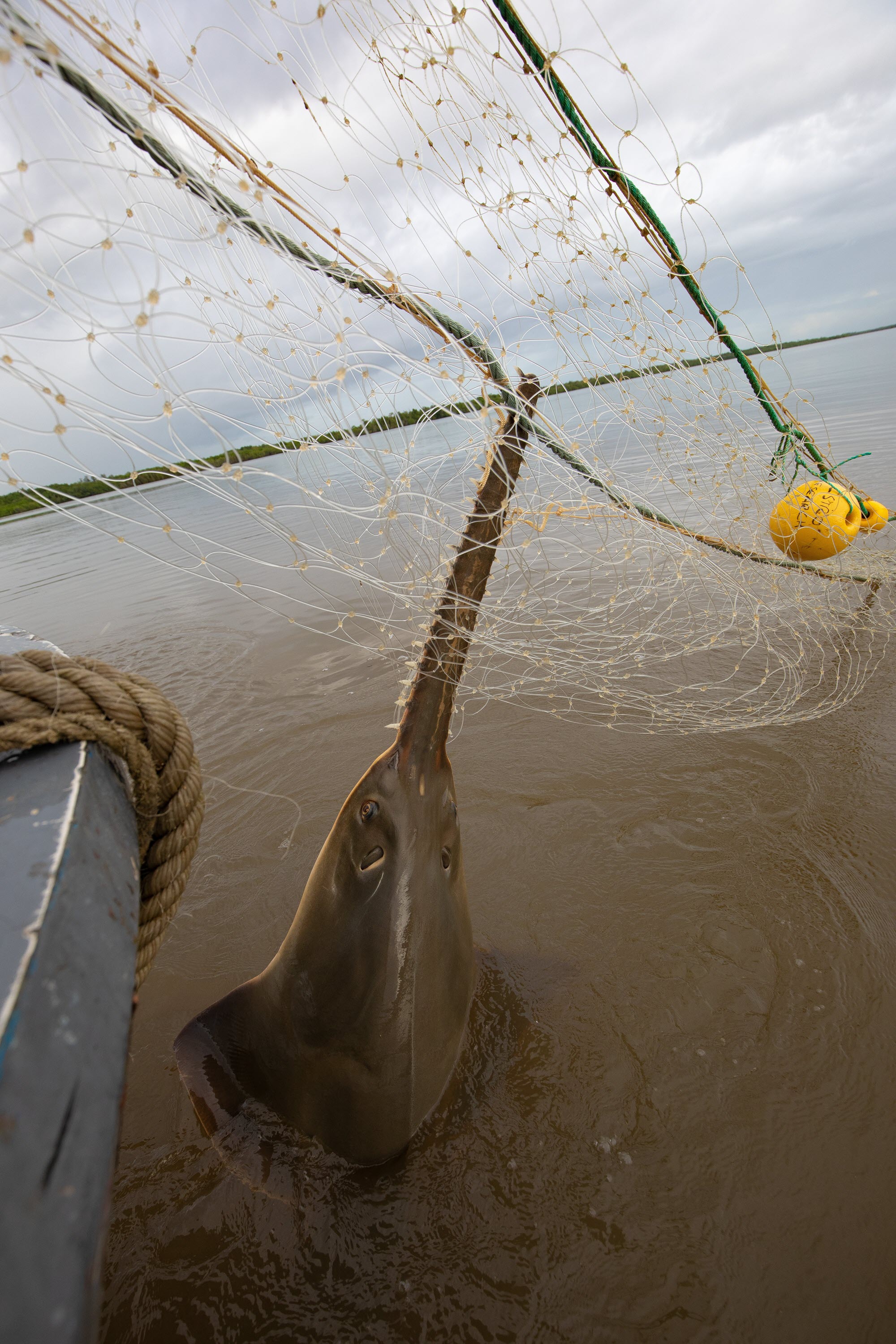
This record provides an overview of the NESP Marine and Coastal Hub project Indigenous Ranger-led monitoring of threatened sawfish in the southern Gulf of Carpentaria. For specific data outputs from this project, please see child records associated with this metadata. This project will partner scientists with First Nations Ranger groups to assess population abundance, distribution and by-catch survival for sawfish species in the southern Gulf of Carpentaria. This project will develop capability in First Nations Ranger Groups that will directly assist with developing baseline status and trends for sawfish species in Australia (including the largetooth sawfish Pristis pristis, which is a priority species: https://www.dcceew.gov.au/sites/default/files/documents/threatened-species-action-plan-2022-2032.pdf). Developing sampling and monitoring capability within First Nations Ranger groups in the southern Gulf of Carpentaria will increase the number of tissue samples for close kin mark recapture (CKMR) population estimates, potentially reducing the present reliance on the fishing industry to collect samples, and ultimately enable sawfish population trajectories to be measured. The CSIRO project team will facilitate capacity building of four Ranger teams within the CLCAC Normanton, Gangaliida and Garawa (Burketown), Wellesley Islands and Ngumari Waanyi (Gregory) to undertake sawfish surveys in the Southern Gulf. The training will build the skills of the Rangers to undertake sawfish surveys to collect tissue samples, distribution data and satellite tagging on CLCAC sea country. Tissue samples collected will contribute directly to the current NESP Sawfish project 3.11 “Multi-fishery collaboration to assess population abundances and post-release survival of threatened sawfish in northern Australia”, which is focused on working with the commercial fishing industry. These samples will be used to obtain baseline estimates of sawfish population status required to monitor population trends. Planned Outputs • Catch data from research surveys and/or indigenous ranger programs (Tabular data) • Tissue samples collected by research and or indigenous ranger programs • Final technical report with analysed data and a short summary of recommendations for policy makers of key findings [written]

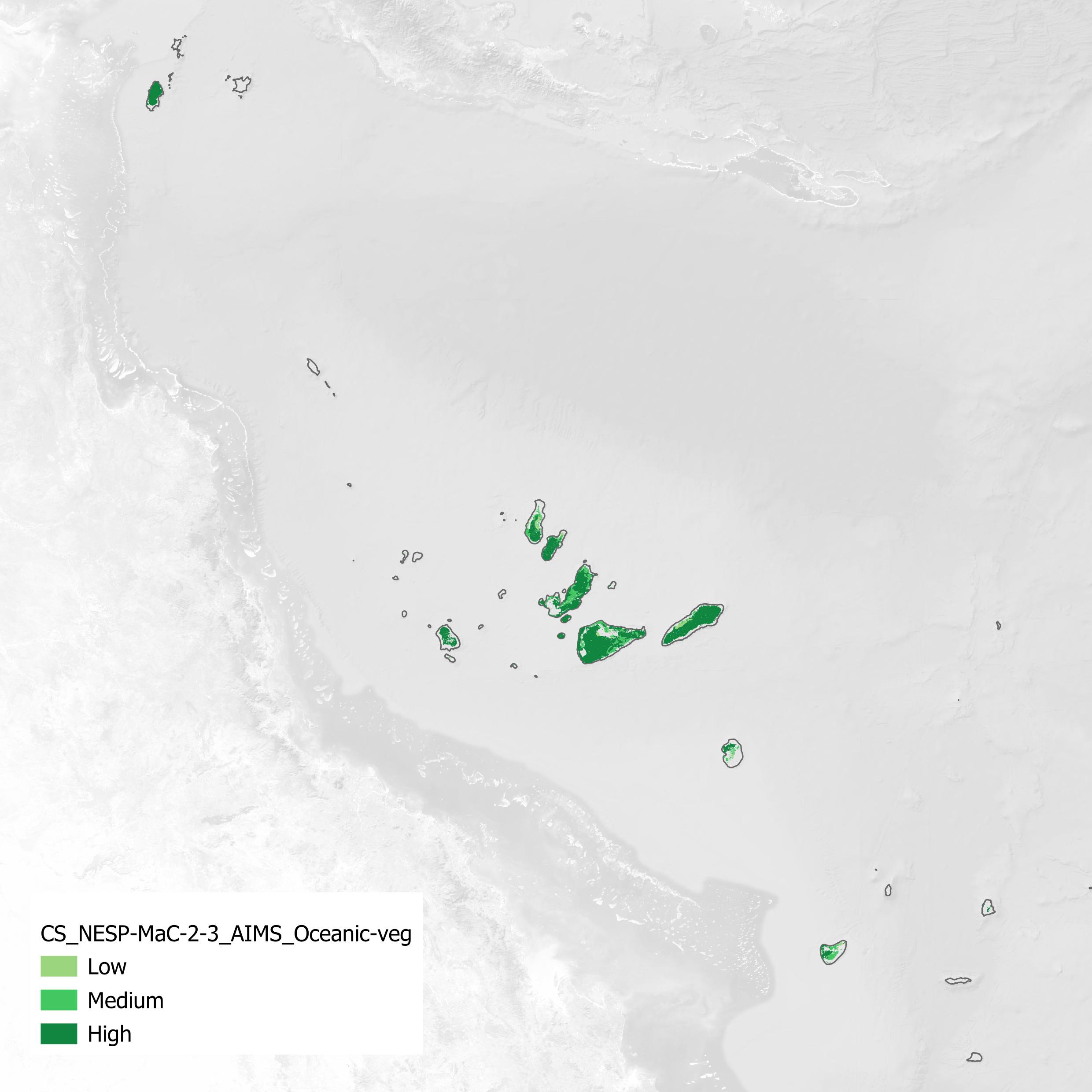
This dataset is a vector shapefile mapping the deep vegetation on the bottom of the coral atoll lagoons in the Coral Sea within the Australian EEZ. This mapped vegetation predominantly corresponds to erect macroalgae, erect calcifying algae and filamentous algae, with an average algae benthic cover of approximately 30 - 40%. Marine vegetation on shallow reef areas were excluded due to the difficulty in distinguishing algae from coral. This dataset instead focuses on the vegetation growing on the soft sediments between the reefs in the lagoons. This dataset was mapped from contrast enhanced Sentinel 2 composite imagery (Lawrey and Hammerton, 2022, https://doi.org/10.26274/NH77-ZW79). Most of the mapped atoll lagoon areas were 45 - 70 m deep. Mapping at such depths from satellite imagery is difficult and ambiguous due to there only being a single colour band (Blue B2) that provides useful information about the benthic features at this depth. Additionally satellite sensor noise, cloud artefacts, water clarity changes, uncorrected sun glint, and detector brightness shifts all make it difficult to distinguish between high and low benthic cover at depth. To compensate for some of these anomalies the benthic mapping was digitised manually using visual cues. The most important element was to identify locations where there were clear transitions between sandy areas (with a high benthic reflectance) and vegetation areas (with a low reflectance). These contrast transitions can then act as a local reference for the image contrast between light and dark substrates. These transitions were often clearest around the many patch reefs in the lagoons which have a clear grazing halo of bare sand around their perimeter. These are often then further surrounded by an intensely dark halo, presumably from a high cover of algae. These concentric rings of light and dark substrate provided local references for the image brightness of low and high benthic cover. These cues also indicated where the hard coral substrate were. These were cut out from this dataset. Validation: Since this dataset was mapped manually from noisy and ambiguous imagery it was important to establish the validity of the visual mapping approach. The manual visual mapping was based on the assumption that the higher the benthic cover of algae, the lower the benthic reflectance. The mapped vegetation therefore corresponded to locations where the benthic reflectance is low, noting that we exclude coral reef hard substrate. To verify if we could reliably map low benthic reflectance areas we first mapped North Flinders and Holmes reefs using visual techniques, then compared this with a direct estimate of benthic reflectance determined by combining the satellite imagery with high resolution bathymetry (Lawrey, 2024, https://doi.org/10.26274/s2a8-nw72). This estimate of the benthic reflectance adjusted the satellite image to the brightness and contrast levels expected for the known depths. This showed there was very strong alignment between the manual visual mapping and low benthic reflectance. The main deviations were with the fine details around reefs, and in some parts where the water clarity made it difficult to determine if the area was vegetation, deep, or water with high CDOM. Unfortunately, the high resolution bathymetry needed for the benthic reflectance estimation was not available for the rest of the Coral Sea and so it was mapped from just the manual visual mapping from the satellite imagery (Lawrey and Hammerton, 2022, https://doi.org/10.26274/NH77-ZW79) based on lessons learnt from North Flinders and Holmes reefs. The final mapped areas in Holmes, Tregrosse and Lihou Reefs were validated against a drop camera survey conducted by JCU in 2022 (yet to be published). From this 219 survey locations overlapped the atoll lagoons. Preliminary analysis indicating that areas mapped in this dataset as having high benthic vegetation typically have 15 - 70% (average 42%) algal benthic cover, typically as a mix of erect macroalgae, erect calcareous algae and filamentous algae. Lagoonal areas that were mapped as sand (i.e. areas outside the mapped vegetation, but not on a reef) typically have a much lower algal benthic cover of 0 - 22% with an average of 4%. These areas were also typically turf algae. Method: To allow the deep benthic features to be seen the blue channel of the image composites was greatly contrast enhanced to show the very faint differences in brightness due to changes in the benthos. The amount of contrast enhancement, and thus the maximum depth that could be analysed was limited by the visual anomalies in the imagery and the magnified variations in brightness across the images due to the following: - Remnant patches from masked clouds. - Remnant patches from cloud shadows that were not fully masked. - Sentinel 2 MSI detector brightness offsets. - Uncorrected tonal change across the full Sentinel swath (western side is brighter than the eastern side). - Coloured Dissolved Organic Matter in the water increases the light attenuation, making areas darker than they would appear in clear water. This tends to occur in areas with low water flushing. - Sensor noise in the imagery. - Remnant sun glint correction due to surface waves. At depth (below ~40 m), only sandy areas are visible as they reflect enough light to be visible above the surrounding visual noise. These sandy areas create a negative space around reefs and patches of dark vegetation, making their shapes visible. Most areas of the coral atoll lagoons are gently sloping meaning that sudden changes in visual brightness are likely due to changes in benthic reflectance, rather than changes in depth. We use this fact to find the visual edge of regions of low benthic reflectance (vegetation). The benthic cover (vegetation, coral or sand) was determined by manual inspection of the contrast enhanced imagery, looking for the following visual cues: - Grazing halos around patch reefs: a pale ring corresponding to bare sand surrounding a textured dark, rounded feature (patch reef). The grazing halo is typically at a similar depth to the surrounding area. This was verified by analysing bathymetry transects across patch reefs in North Flinders reef. The grazing halo therefore serves as a local brightness reference for a high benthic reflectance substrate. Often the grazing halo is surrounded by a dark halo of extra dense vegetation. This dark ring provides a brightness reference for high density vegetation. These brightness thresholds are then used to assess the density of the more distance areas around the reef. If the area is close in darkness to the dark ring around the reef then it is considered high density vegetation. If it is closer to the grazing halo bare sand then it is considered to be free of vegetation. - Reefs without grazing halos: In some cases the patch reefs do not have a pale grazing halo around them. In these cases we identify the reef by its pale circular shape, combined with evidence that it is a tall structure, by checking if it is visible in the green channel (B3), indicating that it reaches within 30 m of the surface or the available bathymetry indicates the vertical nature of the reef. These patch reefs also typically have a dark halo around them, often darker than the surrounding flat lagoonal areas. These dark rings are used as an indication of the brightness level corresponding to high density vegetation. - Low relief flat reefs: In the western side of the Tregrosse reefs platform there are quite a few dark round features that according to the bathymetry have only a limited relief of less than 8 m. These often have a small grazing halo around their border. It is unclear what the exact nature is of these reefs are, however we assume they are reefal in nature and so we exclude them from the vegetation mapping. - On the atoll plains, particularly on the western side of Tregrosse Reefs platform there are large patches of dark substrate that have clearly blank sandy patches, unrelated to the presence of reefs. In these cases the pale patches are assumed to be bare sand and serve as a high benthic reflectance guide. Limitations: This dataset was mapped at a scale of 1:400k, with our goal being to limit the maximum boundary error to 400 m. Where the imagery was clear the mapped boundary accuracy is likely to be significantly better than this threshold. The spacing of the digitised polygon vertices was adjusted to reflect the level of uncertainty in the boundary. Where visibility was good the digitisation spacing was 100 - 200 m. In high uncertainty areas the digitised distance was increased to 500 - 1000 m. The likely boundary error is approximately equal to the vertex spacing. Many of the large areas of vegetation were littered with hundreds of small patches of lower or no vegetation. These areas were cut out as holes in the digitisation where the holes were a feature larger than 200 - 300 m in size. The vegetation areas were categorised into three levels of vegetation density (Low, Medium and High) based on how dark the substrate appeared, relative to the nearby reference indicators (dark halos around reefs, and clear patches of bare sand). In practice the accuracy of this categorisation is probably quite low, as areas where only cut into these different categories at a large scale. It was very difficult to determine the extent of the vegetation in the lagoon of Ashmore Reef. The lagoon appears to have a low flushing rate and a high amount of CDOM accumulates in the lagoon, reducing the visibility to the point were most of the benthos of most of the lagoon is not visible. To help map this reef the full series of Sentinel 2 images was carefully reviewed for tonal differences that indicate the areas of sand and vegetation. Only 20% of the boundary of the vegetation could be accurately determined, the rest of the mapped boundary is speculative. Data dictionary: - Density: Estimated density of the benthic cover in three categories, Low, Medium and High. Sandy areas, or areas with very low cover were not digitised. Comparing this data to preliminary drop camera results indicates that Low and Medium correspond to an average of 30% benthic cover and High an average of 40% cover. - EdgeAcc_m: (Integer) Approximate accuracy of the feature boundary. Note that in this edition of the dataset only very few polygons were individually tagged with accuracy values. The spacing of the polygon vertices is a better local scale measure of the edge accuracy. - EdgeSrc (Edge Image Sources): (String, 255 characters) The source of the imagery used to digitise the feature or refine its boundary. - Type: Type of the feature. In this dataset all features were 'Algae'. - TypeConf: This is the confidence that the features mapped correspond to the type specified. Care was taken to exclude reefs substrate in the mapped areas, however due to the relative coarse scale of the dataset, some sandy areas and reef areas would be included in some of the polygons. - Area_km2: Area of the polygons in square kilometres. - NvclEco: Natural Values Common Language Ecosystem classification for this feature type. All features are 'Oceanic vegetated sediments'. - NvclEcoComp: Natural Values Common Language Ecosystem Complex classification. All features are 'Ocean coral reefs eAtlas Processing: No modifications were made to the data as part of publication. Location of the data: This dataset is filed in the eAtlas enduring data repository at: data\custodian\2022-2024-NESP-MaC-2\2.3_Improved-Aus-Marine-Park-knowledge\CS_NESP-MaC-2-3_AIMS_Oceanic-veg