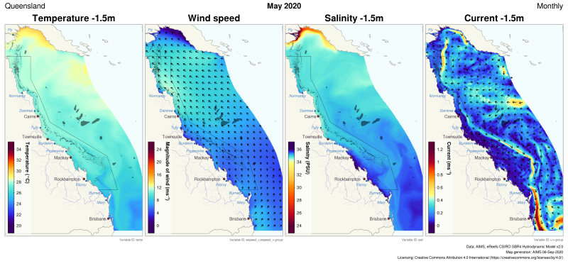
This generated data set contains summaries (daily, monthly, annual) of the eReefs CSIRO hydrodynamic model v2.0 (https://research.csiro.au/ereefs) outputs at both 1km and 4km resolution, generated by the AIMS eReefs Platform (https://ereefs.aims.gov.au/ereefs-aims). These summaries are derived from the original hourly model outputs available via the National Computing Infrastructure (NCI) (https://dapds00.nci.org.au/thredds/catalogs/fx3/catalog.html), and have been re-gridded from the original curvilinear grid used by the eReefs model into a regular grid so that the data files can be easily loaded into standard GIS software. These summaries are updated in near-real time (daily) and are made available via a THREDDS server (https://thredds.ereefs.aims.gov.au/thredds/ ) in NetCDF format. For more information about the eReefs hydrodynamic modelling see https://research.csiro.au/ereefs/models/models-about/models-hydrodynamics/. # Method: A description of the processing, especially aggregation and regridding, is available in the "Technical Guide to Derived Products from CSIRO eReefs Models" document (https://nextcloud.eatlas.org.au/apps/sharealias/a/aims-ereefs-platform-technical-guide-to-derived-products-from-csiro-ereefs-models-pdf ). # Data Dictionary: The following variables are available: - eta: Surface elevation (sea surface height above sea level) (metres) - salt: Salinity (PSU) - temp: Temperature (degrees C) - wspeed_u: Eastward wind (ms-1) - wspeed_v: Northward wind (ms-1) - u: Eastward sea water velocity (second half of the current vector) (ms-1) - v: Northward sea water velocity (half of the current vector) (ms-1) - mean_wspeed: Mean Wind speed magnitude (ms-1) - mean_cur: Mean sea water velocity (current) magnitude (ms-1) # FAQ: ## Why is the mean_cur not equal to the sqrt(u^2+v^2)? The mean_cur is not equal to the sqrt(u^2 + v^2) due to the aggregation process. The instantaneous (raw hourly) u and v values take both positive and negative values as the current changes direction. When these values are averaged over a day or a month, the positive and negative swings tend to cancel out, removing most of the tidal signal. As a result, the aggregate u and v values only show the net current flow. The mean current is different because the current value corresponds to the magnitude of the current, calculated on the hourly data with sqrt(u^2 + v^2). This is then averaged over time. Since the current magnitude is always a positive number there is no ‘averaging out’ of the tidal currents and thus the average is much higher. The daily u and v values show the net current flow (cancelling out any back and forth movement), the mean_cur shows the average current magnitude, i.e. average strength of the net flows and the tidal flows over the period. # How does the regridding work? What algorithm is used? The raw eReefs model (available via NCI) uses a curvilinear grid to minimise the number of simulation cells. This grid format is incompatible with many GIS applications. The products available from the AIMS eReefs THREDDS server are regridded on to a regular rectangular grid. This regridding is performed using an Inverse Distance Weight from the nearest 4 grid cells. A consequence of this approach is that there are an additional set of interpolated pixels along the coastline. Additional detail on the regridding is available in the "Technical Guide to Derived Products from CSIRO eReefs Models". # Depths: This data set contains a subset of the depths available in the source data sets, which differ slightly between the 1km and 4km models. Depths at 1km resolution: -0.5, -2.35, -5.35, -9.0, -13.0, -18.0, -24.0, -31.0, -39.5, -49.0, -60.0, -73.0, -88.0, -103.0, -120.0, -140.0, Depths are 4km resolution:-0.5, -1.5, -3.0, -5.55, -8.8, -12.75, -17.75, -23.75, -31.0, -39.5, -49.0, -60.0, -73.0, -88.0, -103.0, -120.0, -145.0. Limitations: The wind data is originally from the BOM Access-R weather models. These models capture synoptic winds and some of the features of cyclones, however they do not represent the high speed winds near the eye of cyclones well. For this reason the maximum wind speed aggregations do not capture the peak winds of cyclones. The GBR1 yearly summaries of salinity and temperature have a known problem where the data is WRONG with a sharp boundary appearing at edge of the GBR. Do not use this data. We will investigate and resolve the issue with this data. This dataset is based on a spatial and temporal model and as such is an estimate of the environmental conditions. It is not based on in-water measurements, and thus will have a spatially varying level of error in the modelled values. It is important to consider if the model results are fit for the intended purpose.

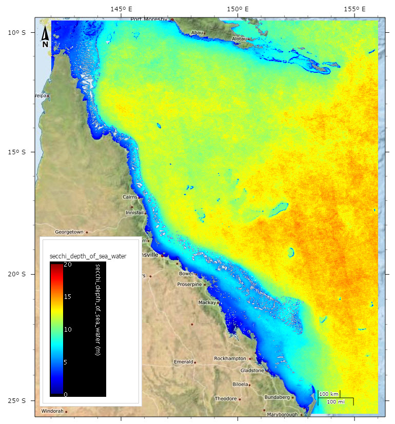
This dataset consists of daily estimates of photic depth on the Great Barrier Reef from MODIS satellite imagery (from 2002 - 2015) using a quasi-analytical algorithm. This algorithm is based on a Type II linear regression of log-transformed satellite and in situ data (2002- 2012). This algorithm was developed as part of data delivery for several NERP projects and was implemented into the NASA SeaDAS tool for processing MODIS imagery. This algorithm and its data products are now routinely run by the Bureau of Meteorology as part of the eReefs Water Quality Dashboard. The data produced from this algorithm were key input datasets for the analysis of NERP TE project 4.1 and integrated as part of the NERP TE 2.3 GBR/TS environmental conditions reports. Method: The satellite imagery was first broken down into its estimated Inherent Optical Properties (IOP) using a quasi-analytical algorithm, outlined in [1]. This process converts the multi-spectral satellite images into an estimate of the various optical properties of the water such as backscattering and absorption of the water. The IOPs were then used to estimate the depth where 10% of the surface light (PAR) level was still available (Z10%). A regression of the in situ ZSD (secchi depth) values against the matching satellite estimates of Z10% was used to adjust the satellite-derived Z10% to ZSD. A Type II linear regression (RMA) of log-transformed satellite and in situ data was used to estimate ZSD for the GBR according to: ZSD = 10^[{log10 (Z10%) - a0}/a1] where a0 and a1 are 0.529 and 0.816 for MODIS-Aqua (N = 71; r2 = 0.83; RMSE = 0.096). The regional tuning parameters a0 and a1 were determined by regression between satellite and in-situ secchi depth measurements from AIMS and QDPI. More details about the methods used to create this dataset can be found in [2]. Format: This data is available in NetCDF raster format from the BOM Marine Water Quality THREDDS server. This server also makes the data available various formats from the following services: OpenDAP, WMS and WCS. http://ereeftds.bom.gov.au/ereefs/tds/catalogs/ereefs_data.html The data for this dataset is available in the mwq P1D Aggregation, mwq P1W Aggregation, mwq P1M Aggregation, mwq P6M Aggregation, mwq P1A Aggregation service end points. These correspond to daily and weekly, monthly, 6 monthly and annual aggregates respectively. The secchi depth estimates correspond to the SD_MIM_* data layers in the service end points. References: 1. Lee, Z.; Carder, K.L.; Arnone, R.A. Deriving inherent optical properties from water color: A multiband quasi-analytical algorithm for optically deep waters. Appl. Opt. 2002, 41, 5755–5772. 2. Weeks, S.; Werdell, P.J.; Schaffelke, B.; Canto, M.; Lee, Z.; Wilding, J.G.; Feldman, G.C. Satellite-Derived Photic Depth on the Great Barrier Reef: Spatio-Temporal Patterns of Water Clarity. Remote Sens. 2012, 4, 3781-3795.

This simulation model allows various scenarios to be run which test how different percentages of nutrient reductions (and the parallel improvement in inshore reef quality) might operate in conjunction with raised water temperatures (as a result of climate change). \n \nThe model has been used for the following simulations: \nThe beneficial impact of end-of-catchment dissolved inorganic nutrients reductions (10%, 30%, 50% and 70%) in raising the bleaching resistance (i.e. the UTBT, °C) of inshore reefs between Townsville and Cooktown. \nThe impact of 10%, 30%, 50% and 70% reductions in end-of-catchment dissolved inorganic nutrients for the Burdekin, Herbert, Tully, Johnstone, Russell, Barron, Daintree, Endeavour, Jeannie and Normanby river systems. \nTwo scenarios for the Tully River Basin - an 18% reduction in fertiliser N application, and a 35% reduction.\n To develop a tool that enables greater characterization of risks posed to the linked GBR social-ecological system due to the effects of climate change.\n The model interfaces source code written in C++ with ArcGIS webmaps. \n \nDetails pertaining to the rationale, development and application of the individual submodels and integrating framework can be found within the refereed journal articles:\n

A one-off study of the effects of handling on Coscinoderma mathewsi around Masig (Yorke) and Kodall (off Masig) Islands. Experimental work was carried out in 2009. \n \nMeasurements of growth (cm) and survival were made to determine how handling might affect sponge growth and survival under aquaculture conditions.\n To determine how handling under aquaculture condiditons might affect sponge growth and survival in Coscinoderma mathewsi.\n

This dataset shows the concentrations of multiple herbicides remaining over time in a simulation flask persistence experiment conducted in 2013. \n \nThe aim of this study was to quantify the persistence multiple herbicides in a standard flask experiment. Time it takes for degradation of half of this herbicide is termed the "half-life". The half-life can be used to help develop environmental risk assessments. \n \n \nMethods: \n \nHerbicide degradation experiments were carried out in flasks according to the OECD methods for "simulation tests". The tests used natural coastal seawater and were carried out in the incubator shakers under 3 conditions: (1) 25°C in the dark, (2) 31°C in the dark and (3) 25°C in the light. The light levels were ~40 µE on a 12:12 light:dark cycle and the flasks shaken at 100 rpm for up to 365 days. \nHerbicides included: \nAtrazine, Diuron, Hexazinone, Tebuthiuron, Metolachlor, 2,4-D, \nWater samples were taken periodically and analysed by high performance liquid chromatography-mass spectrometry (HPLC-MS/MS). \nUncertainty in the analytical method for repeated injections into the LC-MS results in a concentration uncertainty of approximately ± 0.2 µg/L \nReductions in the concentration of herbicides were plotted to predict the persistence of each herbicide (its "half-life"). \nThe emergence of the three herbicide breakdown products were also quantified: Desisopropyl Atrazine and Desethyl Atrazine from Atrazine and 3,4-dichloroaniline from Diuron. \n \n \nFormat: \n \nExcel spreadsheet: Herbicide_persistence_standard_flask_16042015.xlsx \n \n \nData Dictionary: \n \n- Time (days): Time in days from the start of the experiment \n- Sample replicate: Up to three replicate flasks were used containing herbicides and these were incubated under identical light and temperature conditions \n- D25 Atrazine: Concentration of Atrazine remaining in flasks under dark conditions at 25°C \n- D25 Desisopropyl AtrazineAtrazine: Concentration of Desisopropyl AtrazineAtrazine remaining in flasks under dark conditions at 25°C \n- D25 Desethyl Atrazine: Concentration of Desethyl Atrazine remaining in flasks under dark conditions at 25°C \n- D31 Atrazine: Concentration of Atrazine remaining in flasks under dark conditions at 31°C \n- D31 Desisopropyl AtrazineAtrazine: Concentration of Desisopropyl AtrazineAtrazine remaining in flasks under dark conditions at 31°C \n- D31 Desethyl Atrazine: Concentration of Desethyl Atrazine remaining in flasks under dark conditions at 31°C \n- L25 Atrazine: Concentration of Atrazine remaining in flasks under light conditions at 25°C \n- Sample lost: missing data because the sample was lost \n- L25 Desisopropyl AtrazineAtrazine: Concentration of Desisopropyl AtrazineAtrazine remaining in flasks under dark conditions at 25°C \n- L25 Desethyl Atrazine: Concentration of Desethyl Atrazine remaining in flasks under dark conditions at 25°C \n- D25 Diuron: Concentration of Diuron remaining in flasks under dark conditions at 25°C \n- D25 Di Cl Analine: Concentration of 3,4-dichloroaniline remaining in flasks under dark conditions at 25°C \n- D31 Diuron: Concentration of Diuron remaining in flasks under dark conditions at 31°C \n- D31 Di Cl Analine: Concentration of 3,4-dichloroaniline remaining in flasks under dark conditions at 31°C \n- L25 Diuron: Concentration of Diuron remaining in flasks under light conditions at 25°C \n- L25 Di Cl Analine: Concentration of 3,4-dichloroaniline remaining in flasks under light conditions at 25°C \n- D25 Hexazinone: Concentration of Hexazinone remaining in flasks under dark conditions at 25°C \n- D31 Hexazinone: Concentration of Hexazinone remaining in flasks under dark conditions at 31°C \n- L25 Hexazinone: Concentration of Hexazinone remaining in flasks under light conditions at 25°C \n- D25 Tebuthiuron: Concentration of Tebuthiuron remaining in flasks under dark conditions at 25°C \n- D31 Tebuthiuron: Concentration of Tebuthiuron remaining in flasks under dark conditions at 31°C \n- L25 Tebuthiuron: Concentration of Tebuthiuron remaining in flasks under light conditions at 25°C \n- D25 Metolachlor: Concentration of Metolachlor remaining in flasks under dark conditions at 25°C \n- D31 Metolachlor: Concentration of Metolachlor remaining in flasks under dark conditions at 31°C \n- L25 Metolachlor: Concentration of Metolachlor remaining in flasks under light conditions at 25°C \n- D25 2,4-D: Concentration of 2,4-D remaining in flasks under dark conditions at 25°C \n- D31 2,4-D: Concentration of 2,4-D remaining in flasks under dark conditions at 31°C \n- L25 2,4-D: Concentration of 2,4-D remaining in flasks under light conditions at 25°C\n

In March 2007, November 2007 and May 2008, between 6 and 11 sites were surveyed on the coral reefs at Keats Island and Yorke Islands (Masig Island and Kodall Island), in central Torres Strait, to determine the abundance and size frequency patterns of Coscinoderma matthewsi. Sites were located at least 1 km apart and at each site, surveys were conducted at both shallow (4-6 m) and deep (10-12 m) depths, with the former generally on the reef flat. Three 20 x 1 m transects were examined at each depth, with transects separated by at least 20 m to retain independence. For each transect, divers recorded every Coscinoderma matthewsi found within 1 m of one side of the transect line. For each transect, environmental factors such as the degree of reef slope and the percentage of dead coral rubble, sand and consolidated limestone rock, free of living organisms were estimated. For each sponge, the substrate type that it was attached to and growing on was recorded. The habitat in which each sponge was growing was also classified as either exposed (living in an exposed microhabitat, such as on top of rock fully exposed to the ambient water flow) or sheltered (in a sheltered microhabitat, such as under an overhang or protected between surrounding rocks). Sponges were also examined for signs of disease.To examine size frequency distributions patterns, the greatest length, width and height of every Coscinoderma matthewsi was measured with a ruler. For graphical interpretation, sponges were grouped into 2 cm size classes. Some individuals of Coscinoderma matthewsi in Torres Strait have a palmate morphology, where large lobes project upwards from the main sponge base. For each measured sponge, the number of lobes were counted and recorded.\n This research was undertaken to gather further information on the abundance, size frequency patterns and preferred habitat of Coscinoderma matthewsi on the reefs around Keats Island, Masig Island and Kodall Island, where previous surveys indicated that Coscinoderma matthewsi was most abundant. The results of these surveys were compared with previous surveys undertaken under the CRC-TS Project in July 2004, December 2005 and November 2006, to determine whether the abundance of Coscinoderma matthewsi varies around Masig Island over time.\n Keats, Kodall and Masig are sand cays, low-lying (<10 m in height) and small in size (<5 km²). Coral reef surrounds all islands, with broken reef connecting Kodall and Masig. The coral reef slope generally starts at a depth of 6 m (MLW) and stops on sand at 15 m, descending at an angle ranging from 20 to 60°. South-easterly trade winds (15-20 knots) are common from April to December, while monsoonal weather patterns with more northerly winds dominate during summer.\n

A baseline survey of green (no-take) zoned sites and blue (open to fishing) sites in adjacent areas of the northern Great Barrier Reef Marine Park was carried out in December 2006. Three paired sites were surveyed in the Cairns region on deepwater shoals in the vicinity of Green Island and Michaelmas Reef (one green, one blue site off each), and Hastings (Green) and Oyster (blue) Reefs. Assessment of the fish communities was enumerated using baited underwater video sets (BRUVS) and habitat was characterised by towed video. Observations (690) identified 124 species from 33 families, of which 24 species were identified as targeted by fishers. \n \nPrimary substrate (MudSand; Sand; SandCoarse; SandForams; SandHoles; Rubble; Rock; Bedrock; Reef); epibenthic classes (MacroAlgae; Seagrass; Burrowers; FilterFeeders; HardCoral; Isolates; None); and functional units (algae/invertebrates; corallivore; generalist carnivore; generalist; macrocarnivore; herbivore; invertebrate carnivore; macroinvertebrate; carnivore; piscivore; sponges/invertebrates; zooplanktivore) were recorded. \n \nHabitat mapping features assessed from towed video: \nIndividual organisms: Anemone; Ascidian; Bryozoan; Crinoid; Gastropod; Holothurian; Hydroid; Icelet; Solitary Hard Coral; Solitary Soft Coral; Starfish; Urchin \nSubstrate: No Sediment; Soft Mud; Silt - Sandy mud; Sand; Coarse Sand; Sand Rubble Forams; Rubble, 5-50mm; Stones, 50-250mm; Rocks, > 250mm; Reef \nBenthic class: Seagrass (Sparse, Medium, Dense); Algae (Sparse, Medium, Dense); Whip Garden (Sparse, Medium, Dense); Gorgonian Garden (Sparse, Medium, Dense); Porifera (Sponge) Garden (Sparse, Medium, Dense); Hard Coral Garden (Flowerpots - Sparse, Medium, Dense); Live Reef Corals; Caulerpa; Halimeda; Bivalve Shell Beds; Tube Polychaete Beds; Burrowing Animals (Bioturbated Mud); Flora; null.\n To describe the fish fauna in relation to habitat and spatial and temporal variables on selected deep shoals of the GBRMP. \n \nTo present baseline fish community data from BRUVS surveys of three pairs of 'blue' (open to fishing) and 'green' (closed to fishing) zoned shoals in the GBRMP.\n This is one component in a series of surveys conducted as part of this MTSRF project, see also separate metadata records on: \nSouthern mid-shelf Shoals (East and West Warregos; Karamea and Barcoo Banks) \nReef base shoals (Capricorn-Bunker, Pompey and Swains Groups) \nShoals off Cardwell \nMagnetic Shoals (Townsville) \nNote that the 'Northern Shoals' of Cardwell, Cairns, and Magnetic Shoals have individual records as each region was analysed separately. \n \nFish from the following taxonomic classes were recorded (note that not all species/families were recorded at all locations): \nAnguilliformes: Muraenidae (moray eels) \nAulopiformes: Synodontidae (lizardfishes) \nBeryciformes: Holocentridae (squirrelfishes) \nCarcharhiniformes: Carcharhinidae (whaler sharks); Sphyrnidae (hammerhead sharks) \nGasterosteiformes: Aulostomidae (trumpetfishes); Fistulariidae (flutemouths) \nMyliobatiformes: Dasyatidae (stingrays); \nRajiformes: Rhinidae (shark rays); Stegostomatidae (leopard sharks) \nOrectolobiformes: Ginglymostomatidae (nurse sharks); Hemiscylliidae (catsharks); Myliobatidae (manta and eagle rays) \nPerciformes: Acanthuridae (surgeon-fishes); Apogonidae (cardinal fishes); Blenniidae (blennies); Caesionidae (fusiliers); Carangidae (trevallies); Chaetodontidae (butterflyfishes); Cheilodactylidae (morwongs); Echeneidae (suckerfishes); Ephippidae (batfishes); Haemulidae (sweetlips); Kyphosidae (drummers); Labridae (wrasses and tuskfish); Lethrinidae (sweetlip emperors); \nLutjanidae (snappers and sea perches); Malacanthidae (tilefishes); Mullidae (goatfishes); Nemipteridae (threadfin bream); Pinguipedidae (grubfishes); Pomacanthidae (angelfishes); Pomacentridae (damselfishes); Rachycentridae (cobias); Scaridae (parrotfishes); Scombridae (mackerels and tunas); Serranidae (groupers and coral cods); Siganidae (rabbitfishes); Sparidae (sea breams); Sphyraenidae (barracudas); Zanclidae (Moorish idols) \nScorpaeniformes: Scorpaenidae (scorpionfish and lionfish) \nSquamata: Hydrophiidae (sea snakes) \nTetraodontiformes: Balistidae (triggerfishes); Monacanthidae (filefishes and leatherjackets); Tetraodontidae (pufferfish). \n \nWhile not part of the designated objectives, fish size can be delineated from the stereo BRUVs tapes.\n

Data on the general appearance and condition of coral reefs which have been manta towed in the Long Term Monitoring Project (LTMP). The data from 4 reef zones - front (seaward) and back (leeward), and north and south (flanks 1 and 2) - are used to create a web page on each zone for each reef (http://apps.aims.gov.au/reef-monitoring/). \n \n The general condition of the reef is recorded, along with its structural complexity (1 and 2), the percentage of live and bleached coral, the dominant benthic lifeform, and dominant hard coral cover and genus. The general abundance of reef fish and giant clams (Tridacna gigas) is also recorded.\n To provide a broad overview of the reef environment.\n Coral Reef - Zone, Lifeform - Benthic, Relative Frequency, Genus. May include some information on coral disease.\n

Towed Video surveys down to a depth of ~50 m was completed successfully all at the following 9 banks and shoals (Baracuda East and West Shoals, Sheldon Shoal, Wave Governor Bank, Heywood Shoal, Echuca Shoal, Goeree Shoal, Eugene McDermott Shoal, Vulcan Shoal). Sampling involved habitat classification conducted in real-time during the surveys, and taking photographic still image at 10 s intervals for subsequent analysis as the cameras were towed across the shoals at a speed of 1-2 knots. Sampling (as kms of shoal surveyed) was scaled according to the size of the shoals and varied between ~6 km at the smallest shoal (Wave Governor bank) to >40 km at the largest shoal (Heywood Shoals). In total towed video was conducted over ~200 km of the banks and shoals.\n This data was collected as part of the S5 Offshore Banks Assessment Survey component of the Monitoring Plan for the Montara Well Release Timor Sea as agreed between PTTEP Australasia and the Department of the Environment, Water, Heritage and the Arts , 9 October 2009 and was undertaken between 15 March and 17 April 2011.\n

About 50 selected reefs throughout the Great Barrier Reef (GBR) are sampled in the AIMS Long-term Monitoring Project (LTMP). A visual census of fish on fixed transects (3 sites per reef, 5 x 50 m transects per site). Fishes from a list of 191 species, representing 10 families, are counted. \n \nIndividuals, Genus, Species are counted for a prescribed list of 212 species: all the parrotfishes, damselfishes, surgeon fishes, butterflyfishes, and some others. A full list of species observed each year are included in the appendices of each AIMS status report. \n \nIn 2004 a new zoning plan was implemented in the Great Barrier reef Marine Park and in 2006 the pattern of surveys was changed. The original set of reefs (47) are surveyed in odd years (e.g. 2007) and a different set (56 reefs) are surveyed in even years. The new set consists of paired reefs (one no-take, and one open to fishing) surveyed to assess the effects of rezoning. The paired reefs are near Cairns and Innisfail, Townsville, Mackay, the Swain Reefs and the Capricorn-Brunker group. \n \nThe lengths of coral trout only are standardly recorded.\n To detect changes in reef fish communities over time at a regional scale.\n All fish species counted are largely non-cryptic, easily identified underwater and include both commercial and non-commercial taxa. Because surveys span the annual recruitment season, 0+ individuals are excluded from counts: these are distinguished from adults by their small size and often distinctive colouration. \n \nAbundance data for each fish species is subsequently summed over the five transects at each site on each reef to provide reasonable sample sizes for analysis and interpretation. \n \nUpdated results of surveys can be found at: \nhttps://www.aims.gov.au/docs/research/monitoring/reef/latest-surveys.html \n \nA subset of the data has been provided to the Ocean Biogeographic Information System (OBIS, http://www.iobis.org/explore/#/dataset/3936). \n \nData have been used for the e-Atlas: \nhttp://eatlas.org.au/data/uuid/05bde62a-70ec-407b-b999-30cf369498af\n