Australia’s marine estate is vast, with iconic coral reef ecosystems such as the Great Barrier Reef and Ningaloo Reef. However, beyond these famous reefs lie thousands of inshore reefs along Australia's tropical coast, many of which remain poorly characterised or entirely unmapped, leaving them vulnerable due to a lack of targeted protection and management.
Studying these marine habitats is challenging given the scale and isolation of northern Australia. Remoteness, turbid water, strong tidal currents, and the presence of crocodiles limit field work along much of the coast. Satellite imagery provides a low-cost way to build a basic understanding of these shallow marine environments, but this still has significant challenges. Common sources such as Google Maps and ArcGIS Online cover only parts of this seascape, and their sub-surface visibility is highly variable.
The European Space Agency Sentinel 2 satellite images most of Australia’s marine estate every five days at 10 m resolution, but individual scenes are frequently obscured by clouds, sunglint, turbid water and sensor noise.
To overcome these issues, the NESP MaC 3.17 project has produced a new marine-optimised composite of Sentinel 2 imagery that spans the tropical regions of Australia. By stacking and blending tens to hundreds of Sentinel 2 scenes at each location, the process removes most clouds, sunglint and turbidity artefacts, delivering our clearest view yet of these shallow habitats.
Satellite composite image products
This data story highlights the following satellite image products:
- Sentinel 2 All-tide true colour composite imagery – This covers all tropical waters of Australia (except Coral Sea) and is ideal for studying near shore to offshore areas.
- Sentinel 2 Low-tide true colour and infrared composite imagery – This covers the inshore waters of Australia and is ideal for inshore and intertidal areas where the water is turbid. The infrared version can be used to highlight areas that emerge at low tide.
 Eric Lawrey, AIMS
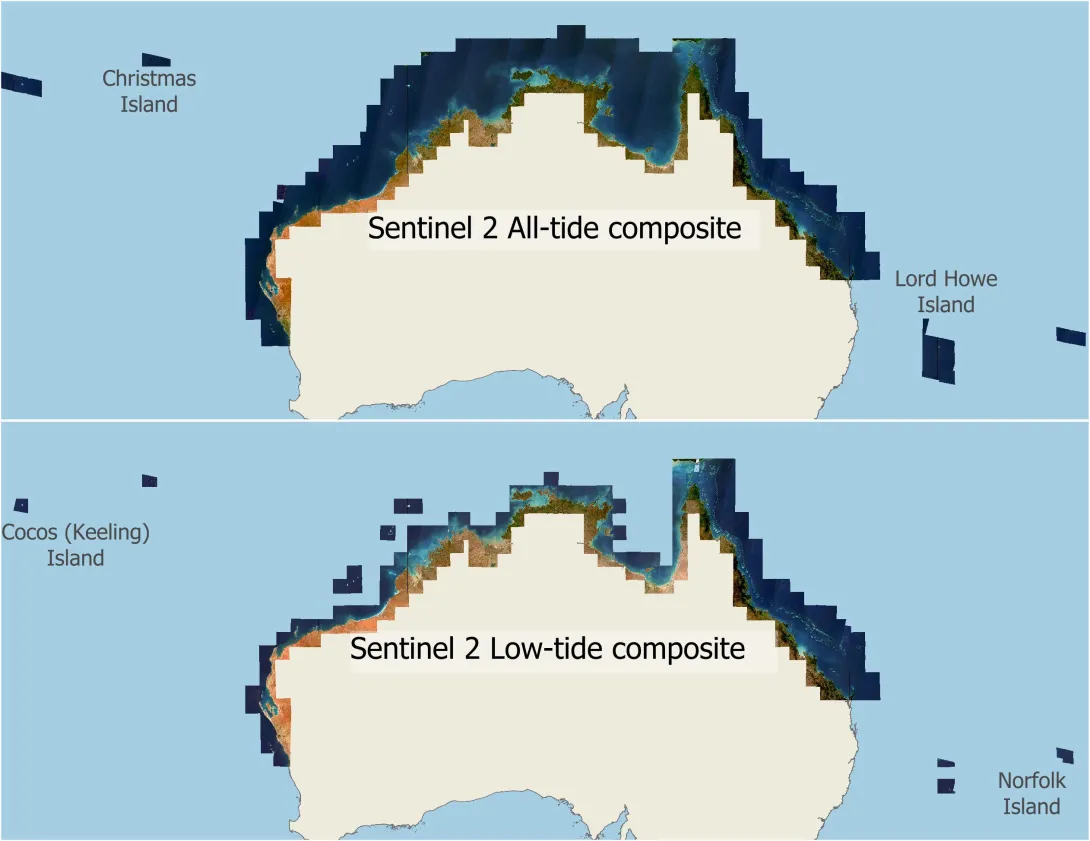
Figure 1. Map showing the extent of the NESP MaC 3.17 Sentinel 2 composite imagery. The All-tide composite covers offshore areas, whereas the Low-tide composite is restricted to nearshore areas, except in the GBR. The imagery also covers remote islands and reefs in the Indian and Pacific oceans, including Cocos (Keeling) Island, Christmas Island, Lord Howe Island and Norfolk Island.
The new imagery does not include the Coral Sea because this region is already covered by the Coral Sea features satellite imagery and raw depth contours (Sentinel 2 and Landsat 8) 2015 – 2021 (AIMS) dataset.
How can I view this imagery?
You can explore the imagery through an interactive map of the Sentinel 2 imagery in the eAtlas or consume them directly in any desktop GIS via the Web Map Tile Service. Look for the following layer names:
- AU: Northern Australian Sentinel 2 composites version 2
- AU: Tropical Australian Sentinel 2 low-tide near-infrared false colour composites
- AU: Tropical Australian Sentinel 2 low-tide true-colour composites.
For detailed analysis, rapid display or custom contrast enhancement, download the full-resolution tiles from the dataset metadata page. They are available as a collection of GeoTiff image files. See ‘FAQ - How do I download the imagery dataset, or just an area I am interested in?’ for instructions.
What can we see?
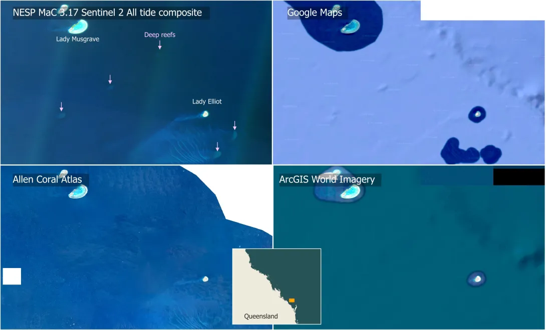
Unlike standard satellite imagery, the new marine-optimised composite imagery is specifically designed for marine environmental applications, revealing benthic features at far greater depths than previously possible. Figure 1 compares the new imagery against existing common satellite image basemaps. Google Maps and ArcGIS World Imagery only cover isolated, very shallow areas. This prevents these map services from being useful for discovering deep reefs. They do however typically provide far higher image resolution in the shallow areas than the Sentinel 2 imagery. The Allen Coral Atlas provides much more complete coverage of the marine coverage but is often too noisy to show deeper features.
In some areas the Sentinel 2 All-tide composite imagery is clear enough to see to the sea floor. This includes the area around the Capricorn Bunker group of reefs, Hervey Bay, and the mid-shelf to outer shelf of the GBR north of Lizard island. Figure 2 shows that between Lady Musgrave and Lady Elliot islands five deep coral reef shoals, 35 – 45 m below the surface, are visible in the All-tide composite imagery, allowing their location, shape and rough structure to be seen. These features are absent from Google Maps, Allen Coral Atlas and the ArcGIS World Imagery.
 Eric Lawrey, AIMS
Figure 2. Sentinel 2 All tide composite imagery verses commonly available satellite basemaps. The new imagery reveals five deep coral reef shoals not visible in the other imagery.
 Eric Lawrey, AIMS
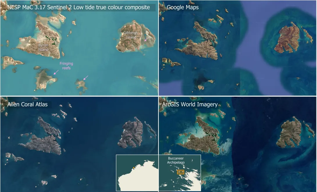
Figure 3. Sentinel 2 Low-tide composite imagery verses other common basemap imagery for a region in the Kimberley. This region has large tides that lead to turbid waters and so reefs are largely invisible except at low tide. The Low-tide composite allows features shows fringing reefs around all the islands, which are mostly invisible in all the other image sources.
Much of the northern and western coastline of Australia has very high tides. These tides stir up sediment, reducing water clarity to less than a metre. Shallow reefs are obscured, except at low tide. Unless the satellite imagery is aligned in time to the low tides then these reefs stay hidden. Figure 3 shows an example in the Kimberley. This location has tides larger than 8 m. Nearly all the islands in this region have fringing reefs, but these are not visible or barely visible in Google Maps, ArcGIS World Imagery and the Allen Coral Atlas imagery. While the Sentinel-2 All-tide composite imagery (not shown) does show these fringing reefs they are not as clear as they could be because the All-tide composite combines images from all tide levels, both low and high tide. This means that for many of the images in the composite the tide is up to 6 - 10 m above the tops of the reefs. Given that the water visibility is at most a couple of metres these reefs are invisible except at low tide. The Sentinel-2 Low-tide true colour composite is tailored to provide the best view of these macrotidal areas. This composite is made up from the ten lowest tide images for each location, resulting in an image that is typically within 1 m of the lowest tide for an area. This reveals shallow features that are completely hidden in imagery not taken at low tide. Because the low-tide imagery is composed from a smaller number of images it has less turbidity smoothing and noise reduction than the all-tide imagery. This makes the low-tide imagery inferior to the all-tide imagery away from the coast, where the largest tides occur.
How was the imagery produced?
The Sentinel-2 All-tide and Low-tide composite imagery were produced by combining many satellite images for each location captured over a nine-year period (2015 - 2024).
The Sentinel-2 pair of satellites (Sentinel-2A, Sentinel-2B) take images of each location on Earth every five days. Most of these single-day pictures are spoiled by clouds, sunglint or murky turbid plumes of stirred-up sediment. These distractions are different in each pass of the satellite, while the seafloor features, such as reefs, are fixed. By merging the images from many dates, we can cancel out the unwanted features and let the faint, stationary reef signals build up.
The processing is achieved with three major steps:
1. Remove cloudy images: we start by throwing away daily Sentinel-2 scenes that are obviously poor, with too much cloud (typically > 20% cloud cover) or strong sunglint.
2. Mask out clouds and use infrared bands to correct for sunglint: the Copernicus cloud-probability layer is used to mask clouds and their shadows from the image, and the sunglint is corrected by subtracting a scaled copy of the infrared band. Infrared light barely enters the water and so over water it mostly just records the sunglint, making it an almost perfect way to correct the imagery. While these steps do not remove every blemish they remove a substantial amount of noise from the image stack.
3. Combine a stack of images: all cleaned images of the same area are stacked, one above the other. For each ground pixel we look down that stack, sorting the brightness values from dark to bright, and the final output is the 15th-percentile value (15% along the sorted values). The darkest readings are usually deep cloud shadows, the brightest are clouds or bright sediment plumes. Picking the low-end 15th percentile gives us a colour that most often comes from clear water on a clear day without dipping into the shadows. Doing this independently for every pixel produces a seamless picture that shows the reefs far more clearly than any single satellite image. The number of images that go into the stack varies from scene to scene. Many offshore areas have fewer images available because not all satellite images are stored in the Google Earth Engine catalogue. Additionally, some areas, particularly those near the equator, have such high cloud cover that almost none of them correspond to low cloud days. As a result, the quality of the composites varies. Some locations are very low noise, while others have lots of cloud anomalies.
 Eric Lawrey, Australian Institute of Marine Science. Source imagery: European Union, contains modified Copernicus Sentinel data 2024, processed with EO Browser
Figure 4. Typical Sentinel 2 daily image on a cloud free day of the Gulf of Carpentaria. Resuspended sediment obscures the view of any reefs in the scene. There are reefs in the top left of the image, but they are not visible in any single daily images due to the low water visibility.
 Eric Lawrey, Australian Institute of Marine Science. Source imagery: European Union, contains modified Copernicus Sentinel data 2024, processed with EO Browser
Figure 5. Combining many satellite images smooths out the turbid plumes, allowing reefs that were invisible in the daily imagery to become visible. The imagery is still hazy and needs contrast enhancement to see these reefs, but it allows previously unmapped reefs to be identified and mapped.
Discovering Hidden Marine Features
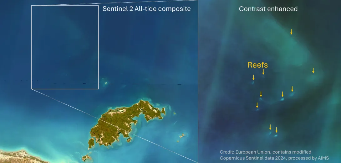
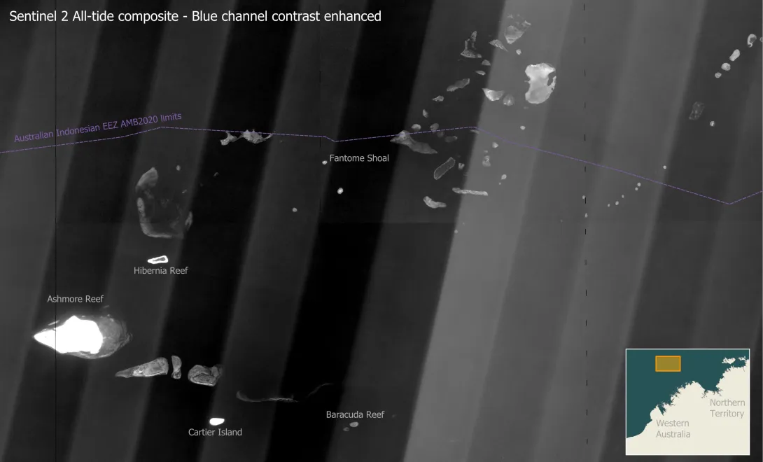
In clear offshore waters of the north west shelf we can see (Figure 6) the deep shoals that formed on the edge of the continental shelf. While some of these banks have been well explored (see Big Bank Shoals of the Timor Sea, and North West Banks and Shoals of the Timor Sea) most of these banks are only known by their bathymetry. The satellite imagery shows patches on these banks where dense algae and hard coral substrate is exposed above the soft sediment that covers most of the area of these banks. This provides clues to the distribution of the habitats on the banks that have not yet been surveyed.
 Eric Lawrey, Australian Institute of Marine Science. Contains modified Copernicus Sentinel data 2024, processed by AIMS.
Figure 6. This map shows the many banks and shoals on the edge of the north west Australian continental shelf. Most of these features are 20 – 25 m deep. At this depth the blue channel of the All-tide satellite imagery provides the best view, with contrast enhancement used to brighten these deep features. Shallow reefs, such as Ashmore and Cartier Island, are blown out white due to the contrast enhancement. Due to the extreme brightening we can also see vertical angled light and dark bands across the imagery. This is caused by each of the 12-part segmented sensor in the Sentinel 2 satellite viewing the scene from a slightly different angle. This banding was not corrected for in the imagery, but is only visible with high levels of contrast enhancement.
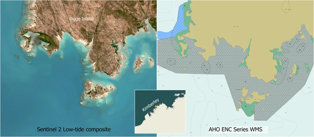
The satellite imagery can also be used to study the inshore coastal areas. Inshore areas are difficult to map by boat as bathymetry scans become very narrow in shallow water. A fair percentage of nearshore coastal areas of the north-west of Australia are uncharted in the AHO marine charts. The satellite imagery provides the opportunity to understand the nature and extent of these nearshore habitats. It should however be noted that the satellite imagery is not suited for navigation as there are likely to be shallow marine hazards that are not visible in the imagery.
 Eric Lawrey, Australian Institute of Marine Science
Figure 7. The satellite imagery can be used to better understand the reefs that exist in uncharted regions. In this example we can see that Bigge Island is fringed by coral reefs. These reefs occur in the uncharted region (grey region with dashes) of the AHO ENC Marine Charts (Jun 2025).
Interactive maps of these satellite composites allow researchers, managers, and the broader community to explore the marine habitats of tropical Australia.
Real-World Applications
The satellite imagery was developed for mapping the reef boundaries and habitats across north and west Australia, as part of the NESP MaC 3.17 project, to provide the most comprehensive catalogue of coral and rocky reefs for this region.
Additionally, researchers from the University of Queensland used the All-tide composite imagery for remapping reef extents of mid-shelf and offshore reefs of the Great Barrier Reef. This remapping resulted in hundreds of deep reefs being added to the reef boundary dataset used by the Great Barrier Reef Marine Park Authority for their management.
Practical Considerations for Users
Although these datasets provide unprecedented clarity, first-time users should approach depth and habitat interpretations cautiously. The marine habitats vary considerably with changes in the environmental conditions, particularly tidal range, turbidity and geological history. Within 10 km of the coastline the visibility is typically less than 10 m, however, in some places such as the Kimberley coastline the visibility is typically less than 5 m. This means that there is still a lot of the marine environment that is not visible in the imagery.
The imagery also only provides a 10 m resolution, making it difficult to pick up texture cues that are important for identifying certain habitat types. Additionally, the colour of benthic habitats changes dramatically with depth.
It is always best to obtain as many in-situ observations as possible to ground truth your interpretation of the imagery for a region. If no in-situ information is available then use what high-resolution imagery is available (drone footage, aerial imagery, high-resolution satellites imagery) of nearby locations to understand the local conditions.
Conclusion
The NESP MaC 3.17 Sentinel 2 composite imagery shows that developing image processing pipelines specifically for the marine environment allows us to see deeper into the water column than ever before. This is, however, not the end of the story. The current imagery only provides a view of the shallow portions of the marine environment and so there is much still to be discovered. With a longer time series of satellite imagery, and smarter methods for combining those images, we expect that further improvements can be made to the clarity of the imagery.
Frequently Asked Questions (FAQ)
How deep can features be detected in the satellite imagery?
The depth that features can be seen in the imagery varies greatly with the water clarity, which is determined primarily by suspended sediment, and Coloured Dissolved Organic Matter (CDOM). In areas shallower than approximately 20 - 30 m, waves and tidal currents stir up the sediment on the sea floor, making the water turbid. These sediment particles scatter the light, making the waters appear brighter due to the reflected light from the sediment. It also blocks the light, reducing the amount of reflected light off the bottom, weakening the reflected view of the sea floor. In macro-tidal areas, such as inshore areas along the Kimberley coast, the turbidity can limit the visibility to as low as a couple of centimetres. An added factor limiting the depth visibility of the imagery is the amount of CDOM in the water. CDOM is generally highest in areas where there are high nutrient levels. CDOM has a ’tea-like’ colour that absorbs light passing through the water. This also limits light passing through the water reducing the amount of reflected light off the sea floor. Areas can have both high CDOM and high turbidity making observing the features to any significant depth extremely difficult.
In clear oceanic areas, the depth visible in the Sentinel 2 All-tide imagery varies from 25 - 60 m depending on the level of Coloured Dissolved Organic Matter in the water. The Coral Sea has the highest visibility, close to 60 m, while on the outer edge of the north-west shelf the visibility is lower, approximately 35 - 45 m. Closer to shore the visibility drops significantly due to high levels of suspended sediment in the water. While the process of combining many images to make a composite image improves the final image significantly, it only smooths out the effects of turbidity eddies. The imagery still has limited depth visibility. At 20 km from the coast the visibility is typically 10 - 15 m. In the inshore the visibility is limited by the turbidity of the water, which varies from a couple of centimetres to 10 m. In general, areas with high tidal ranges tend to be highly turbid leading to poor depth visibility. To combat this, the Low-tide imagery removes 1 - 4 m of water, allowing reef features in these turbid areas to be studied.
Why use the 15th and 30th percentiles – what is the trade-off?
To build each composite we stack many daily Sentinel-2 images of the same spot, line them up pixel by pixel, then pick one value from that stack as our “best guess” of the true colour. Using the average does not work well: a single bright cloud or dark cloud shadow can pull the mean far from the ideal estimate. Instead, we sort the values from darkest to brightest and take a chosen percentile. This keeps most good observations and ignores the extremes.
Clear, sediment-free water is usually darker than turbid water or cloud. So, to pick brightness values that correspond to daily images when the water clarity was higher, we use a percentile threshold below the median (50th percentile). Go too low, though, and we end up with very few contributing images, leading to noisy results and we tend to pick up dark cloud shadow artefacts.
15th percentile (all-tide composites). Because these stacks have dozens of dates, we can afford to use a low percentile such as 15th percentile point.
30th percentile (low-tide composites). Low-tide stacks hold only up to ten images. Choosing the 15th percentile level here would mean relying on just one or two images per pixel, which would lead to noisy results. The 30th percentile level is a safer compromise that still leans toward the clearer scenes while drawing on more data.
What licensing and attribution apply when publishing figures or web maps?
Both composites are released under a Creative Commons Attribution licence (CC-BY-4.0). Any derivative map, graphic or analysis must cite the dataset DOI and acknowledge the Copernicus Sentinel programme and the AIMS processing team. A compact caption line such as “Contains modified Copernicus Sentinel data 2015-2024 processed by AIMS (https://doi.org/10.26274/HD2Z-KM55)” is recommended. Where the dataset is used for a derivative analysis product, the dataset should be cited in the bibliography.
Sentinel-2 All-tide composite imagery:
Hammerton, M., & Lawrey, E. (2024). North Australia Sentinel 2 Satellite Composite Imagery - 15th percentile true colour (NESP MaC 3.17, AIMS) (2nd Ed.) [Dataset]. eAtlas. https://doi.org/10.26274/HD2Z-KM55
Sentinel-2 Low-tide composite imagery:
Hammerton, M., & Lawrey, E. (2024). Tropical Australia Sentinel 2 Satellite Composite Imagery - Low Tide - 30th percentile true colour and near infrared false colour (NESP MaC 3.17, AIMS) (1st Ed.) [Dataset]. eAtlas. https://doi.org/10.26274/2bfv-e921
Will annual updates be released?
The All-tide and Low-tide composites are one-off datasets developed for the NESP MaC 3.17 project. No updates are planned, however, should these datasets be improved on then these new versions will be linked to from these existing datasets.
How do I download the imagery dataset, or just an area I am interested in?
Downloading the full dataset requires 203 GB of storage (All-tide 85 GB, Low-tide true colour 68 GB, Low-tide infrared 50 GB) but provides the fastest access to the imagery. The datasets are available from the eAtlas NextCloud file server, which is linked to from each dataset metadata.
Sentinel-2 Low-tide true colour and infrared imagery - metadata
Sentinel-2 All-tide true colour imagery - metadata
The eAtlas Nextcloud provides the ability to download individual scene images, or the whole dataset as a single giant download. Do not attempt to download the whole dataset in a single go, as any disruption to the download will force you to have to start again. To download the full dataset it is recommended that you use the download-aims-s2.py script. This script allows the download to be resumed after any disruptions. This script also allows individual images or collections to be downloaded.
The imagery is organised using the standard Sentinel-2 UTM tiles, with each image approximately 110 km across. Each grid cell is identified by a 5-character Tile ID, such as 51KUA. This Tile ID also appears in every composite image filename. That ID is all you need to fetch the matching GeoTIFF from the download repository. There is also a Preview gallery that allows relevant imagery to be located visually.
To work out the Tile ID for an area of interest, you can use the Sentinel-2 UTM Tiling Grid interactive map.
Why do some offshore tiles still look noisy even after compositing?
Persistent cloud belts over Christmas Island, Norfolk Island, Lord Howe Island and parts of Torres Strait leave very few clear scenes and so the composition has less material to average over. The outcome is a grainier surface with small flecks of residual cloud artefacts.
Where should feedback or derived layers be sent?
Email either lead author (addresses in the metadata) with a short description of the issue or product. Corrections will be logged in an erratum section of the eAtlas metadata record. Any derivative layers can be listed as related resources so future users can discover them.
How can I stitch multiple Sentinel-2 tiles together?
Once you have the necessary GeoTIFFs, create a virtual raster (VRT). In QGIS choose Raster – Miscellaneous – Build Virtual Raster and point to all the files. The resulting .vrt file can be styled like a single image.
Can this imagery track shoreline changes?
No. Each composite blends scenes collected over six to ten years, so transient erosion or accretion signals are smeared. For shoreline changes, see the Geoscience Australia Digital Earth Australia Coastlines dataset (https://www.ga.gov.au/scientific-topics/dea/dea-data-and-products/dea-coastlines).
Can this imagery show changes in habitats?
No. The composite imagery is an ‘average’ over a long period of time and thus does not show changes in time. Comparing the Low-tide images and the All-tide images shows changes in dynamic habitats such as seagrass and macroalgae. This is due to the different collection of image dates between the two image composites. This difference between the images is, however, an unreliable measure of change over time.
How does this imagery compare to the Allen Coral Atlas?
The Allen Coral Atlas mosaics are built from daily PlanetScope frames. They deliver four-metre resolution but carry more image noise than Sentinel-2 imagery. The 10 m composites presented here are a combination of tens to hundreds of daily images per pixel, yielding clearer benthic texture and up to 50% better depth visibility.